High-Performance GEMM for Deep Learning: From Data Locality to Microkernels

Implementing highly efficient matrix multiplication routines that approach peak performance demands significant effort, strong linear algebra knowledge, and a deep understanding of the underlying hardware architecture (even down to the microarchitectural level[23]). This is why vendors provide highly optimized implementations of the Basic Linear Algebra Subprograms (BLAS)[1], including General Matrix Multiplication (GEMM). GEMM optimization do not perform matrix product naively and instead cast matrix multiplication in terms of rank-1 updates, i.e., outer products \(x \otimes y = x y^t\) which can be decomposed into a sequence of AXPY operations of the form \(y \mathrel{+}= \alpha x\), where \(x, y \in \mathbb{R}^n\) and \(\alpha \in \mathbb{R}\). Each AXPY requires \(n\) fused multiply-add (FMA) operations, i.e., \(2n\) floating-point operations, leading to a total of \(2n^3\) flops for multiplying two \(n \times n\) matrices. In high-performance implementations, the loop over these rank-1 updates is realized as an optimized, architecture-specific microkernel. Microkernels update a small tile of \(C\), kept entirely in registers, by multiplying micro-panels of \(A\) and \(B\). They are carefully designed to exploit vector hardware or units[2], allowing multiple data elements to be processed per instruction and significantly improving throughput.

Beyond the microkernel, performance is achieved through loop transformations and multi-level tiling that target different levels of the memory hierarchy (registers, L1, L2, and L3 caches). The goal is to minimize data movement. In fact, while processors can perform floating-point operations extremely fast, matrix multiplication only reaches high performance when data reuse translates into locality (e.g when loops are localized). Additional optimizations include prefetching [7] to overlap computation and data movement, and loop unrolling [8] to expose instruction-level parallelism and reduce control overhead.

This post is the first in a series dedicated to high-performance programming for scientific computing, machine learning, and deep learning applications. We will study both fundamental optimization techniques and high-quality open-source implementations such as OpenBLAS. In practice, it is often best to express computations in terms of such libraries in order to benefit from the extensive expertise embedded in them (instead of trying to implement it on your own).

To motivate this post, let us consider a simple matrix multiplication using PyTorch, i.e., \( C \mathrel{+}= AB \), where \( A \), \( B \), and \( C \) are square matrices of size \( N = 2^{11} \). A matrix multiplication of the form \( C \mathrel{+}= AB \) requires \( N \) fused multiply--add (FMA) operations for each of the \( N^2 \) output elements, yielding a total of \( 2N^3 \) floating-point operations (FLOPs).

def bench_torch(N):
    A = torch.rand(N, N, dtype=torch.float64)
    B = torch.rand(N, N, dtype=torch.float64)

    for _ in range(warmup):
        _ = torch.matmul(A, B)

    start = time.perf_counter()
    for _ in range(iterations):
        C = torch.matmul(A, B)
    end = time.perf_counter()

    avg_time = (end - start) / iterations
    gflops = (2 * N ** 3) / (avg_time * 1e9)
    return gflops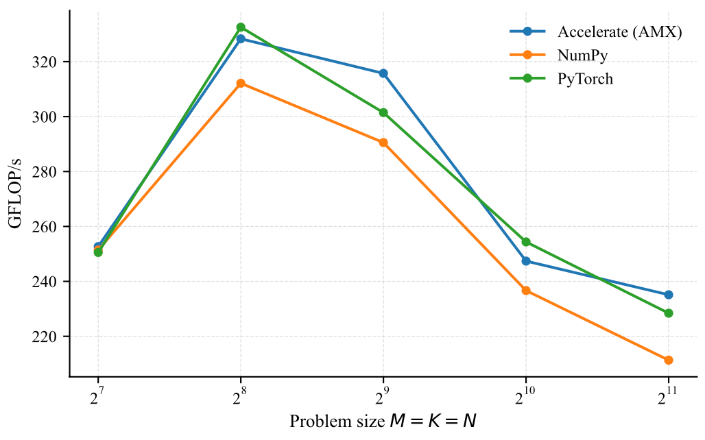

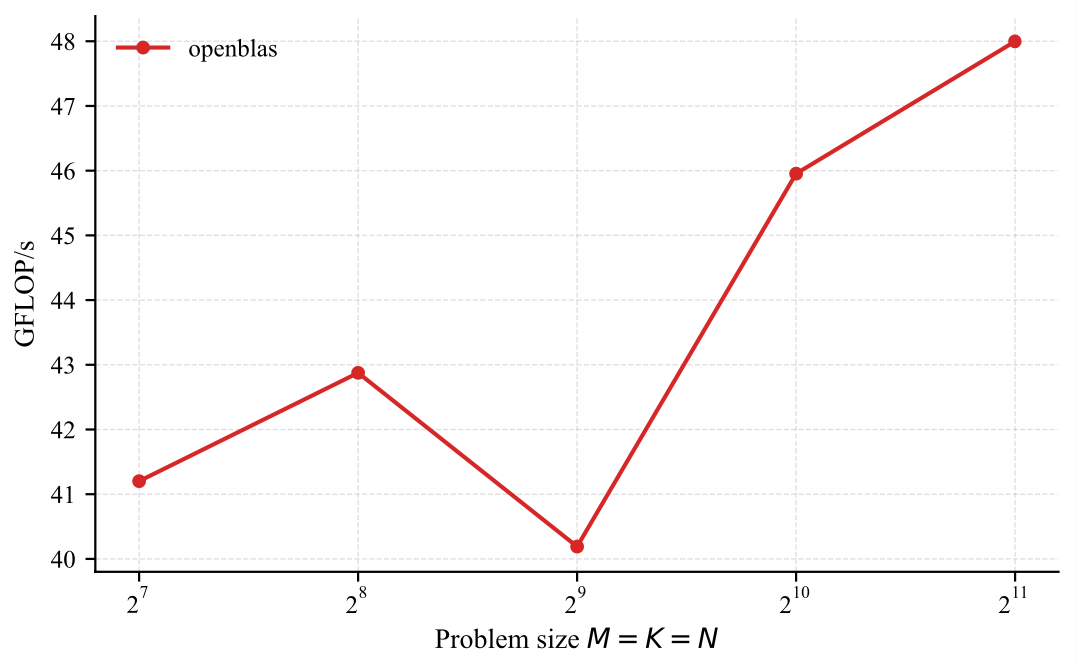
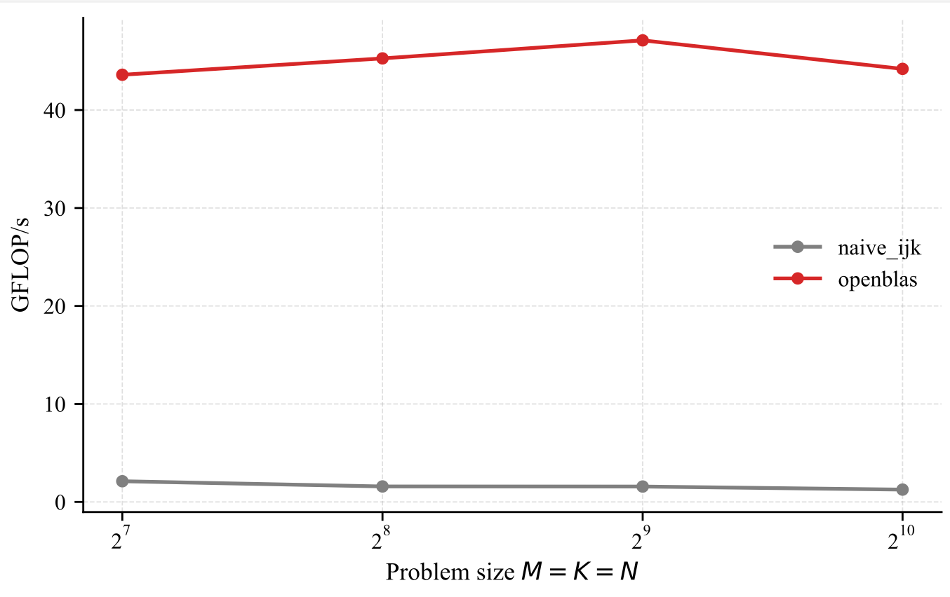
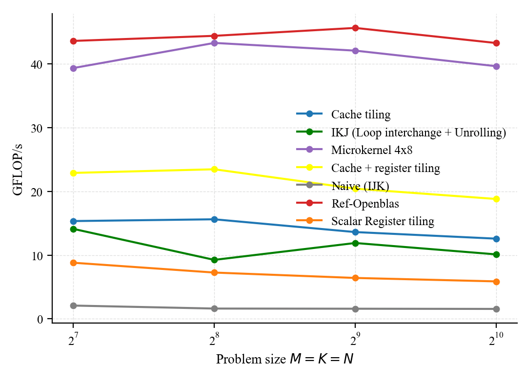
For \( N = 2^{11} \), this corresponds to \( 2^{34} \) FLOPs. Running this computation with PyTorch on an Apple M1 machine takes approximately \( 0.081 \) seconds, which corresponds to about \( 2.12 \times 10^{11} \) FLOPs per second, i.e., \( 212 \)~GFLOP/s. This is very high. Assuming a cpu clock frequency of \( 3.2 \)~GHz, this translates to approximately \( \frac{2.12 \times 10^{11}}{3.2 \times 10^{9}} \approx 66 \) FLOPs per cycle. For a 4-core processor, this corresponds to roughly \( 16 \) FLOPs per cycle per core. Under the hood, PyTorch delegates GEMM to highly optimized libraries (in this case, Accelerate) after releasing the GIL.

From now on, we will use OpenBLAS [21] as our reference (single threaded) implementation. Its performance is depicted below.

Introduction

Matrix multiplication lies at the heart of scientific computing and deep learning, including modern architectures such as transformers. One of the goals of this post is to present the foundations of high-performance GEMM design, including the key parameters that drive performance. In particular, we examine how Level-3 Basic Linear Algebra Subprograms (BLAS) kernels are implemented, as well as numerical kernels in general.

BLAS was basically introduced to define a standard interface for dense linear algebra routines that researchers or developers can invoke in their applications. It promotes portability of high-performance implementations, as each platform may provide its own highly optimized version. As said briefly before, GEMM routines are carefully tuned for specific hardware architectures, where memory is organized as a multi-level hierarchy, and access cost (in cycles) increases with each level. Lower-level caches offer lower latency but smaller capacity.

High-performance implementations aim to fully exploit hardware features such as vector units and multi-threading to accelerate computation and approach peak performance. A key objective is to maximize the time spent in the architecture-specific microkernel while ensuring that reused data remains in cache across iterations, thereby enjoying locality.

Deep learning workloads, including large language models (LLMs), transformers, and fully connected layers, rely heavily on matrix operations during both training and inference. They typically involve a mix of GEMM and GEMV operations, where GEMM is compute-bound and GEMV is memory-bound.

Consider a fully connected layer defined by a weight matrix \( W \in \mathbb{R}^{m \times d} \) and a bias vector \( b \in \mathbb{R}^{m} \), mapping an input \( x \in \mathbb{R}^{d} \) to an output \( y \in \mathbb{R}^{m} \) via \( y = W x + b \). This computation requires \( m \times d \) fused multiply-add (FMA) operations, i.e., \( 2md \) floating-point operations (FLOPs). When processing a batch of inputs, this generalizes to \( Y = W X + b \mathbf{1}^T \), where \( X \in \mathbb{R}^{d \times n} \), each column of \( X \) corresponds to a sample, and \( \mathbf{1} \in \mathbb{R}^{n} \) is a vector of ones. Backpropagation can also be expressed in terms of GEMM operations. After the linear transformation, a nonlinearity is often applied: \( Y = \sigma(Y) \) (otherwise your can not cope with non linear problems). Transformer architectures [9] make extensive use of self-attention and feedforward layers, which can largely be expressed as GEMM operations. During training, most computations can be reformulated as GEMM (e.g., via masking), making training predominantly compute-bound. In contrast, inference in large language models involves a mix of GEMM and GEMV operations. GEMM is primarily used during the prompt prefill phase[9], where input tokens are processed in parallel. Subsequent token generation relies on the key-value (KV) cache and follows an autoregressive process. Since the number of generated tokens is typically large, inference becomes dominated by GEMV operations, which have lower arithmetic intensity than GEMM. As a result, inference is generally memory-bound.

In this post, we present techniques for optimizing matrix multiplication kernels so that they become compute-bound and approach peak performance on CPU architectures by reducing data movement across the memory hierarchy. We consider both macro-level optimizations (such as loop transformations and tiling) and micro-level optimizations (such as microkernel design) to achieve data locality and efficient use of the memory hierarchy. A subsequent post will focus on GEMM and GEMV optimizations for GPU architectures.

The Roofline Model

Modern processors are incredibly complex. At the microarchitectural level, many techniques are employed to hide latency and increase throughput. These include caches, instruction and data pipelining, register renaming [10], and out-of-order execution. Additionally, multicore architectures are used to further increase peak performance and exploit thread-level parallelism.

source: https://en.wikipedia.org/wiki/Roofline_model

While hardware evolves to compute FLOPs very fast, organizing computational kernels to exploit all these features and get close to peak performance is not trivial and requires significant effort. This includes loop unrolling to increase ILP, SIMD [11] to reduce fetch and decode overhead, balancing floating-point operation mix to exploit FMA units (e.g., parity between MULTs and ADDs), prefetching[7] to overlap computation and data movement, and reduction of memory traffic so that kernels approach the compulsory memory traffic.

For example, using good stride access enables spatial locality, reuse enables temporal locality, and organizing data avoids conflict misses (e.g., padding arrays using cache arithmetic) during hotspots. Especially important is distributing the data on which computation kernels operate across different memory layers, i.e., register and cache tiling or multi level tiling.

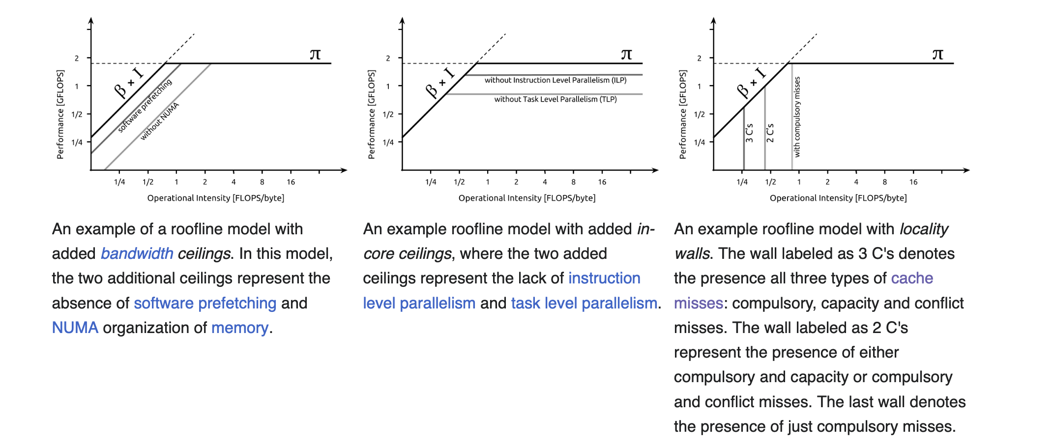
Naturally, all of this exacerbates the difficult job of engineers who seek to understand the primary factors affecting the performance of a floating-point kernel, i.e., which optimization yields the highest benefit. One way to understand how to optimize code and make it run faster is to look at the operational intensity \(I\), defined as the ratio of compute to memory traffic, which tells us which ceilings to consider.

Let \(C\) denote the number of cycles spent on some kernel, \(F\) the number of FLOPs, and \(L\) the number of bytes loaded. Let \(\pi\) be the attainable peak performance (e.g., FLOPs per cycle) and \(\beta\) the memory bandwidth (bytes per cycle). If we assume that computation and data movement (traffic between caches and memory rather than between core and caches) cannot be overlapped, then the number of cycles required is \(C = \frac{F}{\pi} + \frac{L}{\beta}\). To compare the relative contribution of computation and memory traffic, we rewrite both terms with a common factor \(\frac{1}{\beta} \): \(C = \left(\frac{F\beta}{\pi}\right)\frac{1}{\beta} + L \cdot \frac{1}{\beta}\). Thus, if \(L >> \frac{F\beta}{\pi}\) then the cycles are dominated by memory, i.e., the kernel is memory-bound. This also implies \(I \beta < \pi\) where \(I = \frac{F}{L}\) is the arithmetic or operational intensity.

In practice, computation and data movement can overlap to some extent. This leads to the bound \( \max\left(\frac{F}{\pi}, \frac{L}{\beta}\right) \leq C \leq \frac{F}{\pi} + \frac{L}{\beta}\). In the ideal case of perfect overlap, we obtain: \(C = \max\left(\frac{F}{\pi}, \frac{L}{\beta}\right)\). Thus, the performance (FLOPs per cycle) is:

\(P = \frac{F}{\max\left(\frac{F}{\pi}, \frac{L}{\beta}\right)} \leq \pi\)

\(P = \frac{1}{\max\left(\frac{1}{\pi}, \frac{L}{F\beta}\right)}\)

\(= \min\left(\pi, \underbrace{\frac{F}{L}}_{I:= \text{arithmetic intensity}}\beta\right)\)

\(= \min\left(\pi, I\beta\right)\)

This shows that performance is limited either by compute capability \(\pi\) or by memory bandwidth scaled by arithmetic intensity \(I\beta\). If \(I > \frac{\pi}{\beta}\) then \(I\beta > \pi\), and performance can attain the peak \(\pi\), meaning the kernel is compute-bound. The term \(\frac{\pi}{\beta}\) is known as the ridge point [12], i.e., the minimum intensity required to achieve peak performance. On the other hand, low operational intensity (\(I < \frac{\pi}{\beta}\)) implies the kernel is memory-bound, i.e. sufficiently high intensity means compute-bound, while relatively low intensity means memory-bound. Before the ridge point, performance grows linearly with intensity with slope \(\beta\) i.e \(P = \beta I\) and after the ridge point, performance saturates at \(\pi\). Increasing intensity can move a kernel from the memory-bound regime to the compute-bound regime.

The roofline model, involving both computational and bandwidth complexity, is widely used in deep learning to understand bottlenecks in kernels such as GEMM and GEMV. For example, LSTM [13] kernels typically exhibit lower FLOP/s performance and higher data movement compared to convolutions or transformers due to limited parallelism.

Finally, let’s stress again that the roofline model is an optimistic model; it assumes that compute time can overlap with bandwidth time. In practice lower ceilings are hit and thus the model provides an upper bound on achievable performance.

Loop Nests, Locality, and Cache Arithmetic

A cascade of loops, i.e., a set of loops nested inside one another, is called a loop nest[14]. A loop nest is perfectly nested when the assignments are all hosted in the innermost loop (e.g matrix multiplication). An example of an imperfectly nested loop is Cholesky factorization [3]. The set of nested loops that accesses a volume of data not exceeding the cache size is referred to as the localized iteration space.

What is important to understand is that reuse does not necessarily imply locality (i.e., cache hits). Data locality can be characterized, in the polyhedral model [4], as the subset of iteration space directions along which data reuse results in cache hits which can be obtained by intersecting the data reuse vectors with the localized iteration space. For example, consider the (ikj) algorithm for matrix multiplication. When the matrices are large, the localized iteration space is \(\mathrm{span}(0,0,1)\) only.

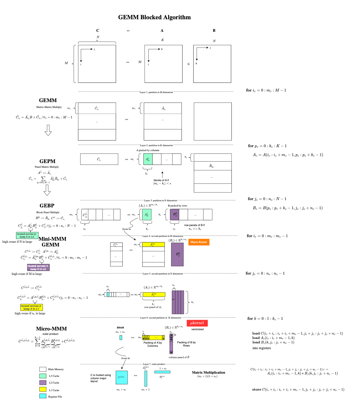
Let \(A\), \(B\), and \(C\) denote matrices in \(\mathbb{R}^{M \times K}\),\(\mathbb{R}^{K \times N}\), and \(\mathbb{R}^{M \times N}\) respectively, with entries \(a_{ik}\), \(b_{kj}\), and \(c_{ij}\). For simplicity we assume that \(M= m_cM'\), \(N = n_cN'\), and \(K = k_cK'\), i.e \(M,N\) and \(K\) are multiples of \(m_c,n_c\) and \(k_c\) respectively. If we consider an \(l \times d\) submatrix \(A_{ld}\) of a matrix \(A\), then, if \(l\) and \(d\) are approximately equal, \(A_{ld}\) is said to be a block of \(A\), else if \(d \gg l\), then \(A_{ld}\) is called a row panel, and if \(d \ll l\), then \(A_{ld}\) is called a column panel of \(A\).

Regarding how arrays are mapped to memory, we assume that matrices are linearized in memory using a row-major layout. Let \(A\) be an \(n\)-dimensional array where \(\text{s}_k\) denotes the number of elements in dimension \(k\), and consider a loop nest of depth \(m\) represented by the iteration vector \(\vec{i}\). The row-major layout mapping \(a\) is a function \[ a : \mathbb{N}^m \rightarrow \mathbb{N} \] of the loop indices: \[ a(i_1, \ldots, i_n) = \text{offset} + i_1 \cdot \text{s}_2 \cdots \text{s}_n + i_2 \cdot \text{s}_3 \cdots \text{s}_n + \cdots + i_{n-1} \cdot \text{s}_n + i_n . \] where \(\text{offset}\) denotes the base address of the array \(A\), i.e. its displacement in memory. Thus the memory address of an element of array \(A\) (i.e. a reference) can be written as \[ \text{Memory\_Address\_of\_A}[i_1, \ldots, i_n] = \text{Mem}_{R_A}(\vec{i}) = a(i_1, \ldots, i_n). \] The cache set accessed by the reference \(R_A\) is given by \[ \text{Cache\_Set}_{R_A}(\vec{i}) = \underbrace{\left \lfloor \frac{\text{Mem}_{R_A}(\vec{i})}{L_s} \right \rfloor}_{Mem^{L}_{R_A(\vec{i})}} \bmod N_S \] where \(L_S\) denotes the cache line size and \(N_S\) the number of cache lines. We have a cache interference (self or cross) when the cache set accessed by \(R_A\) at \(\vec{i}\) is the same as any of the cache sets accessed by \(R_B\) at every potentially interfering iteration \(\vec{j}\) between \(\vec{p}\) and \(\vec{i}\) i.e when \[ \text{CacheSet}_{R_A}(\vec{i}) = \text{CacheSet}_{R_B}(\vec{j}) \] which implies \[ \text{mem}_{R_A}^{L}(\vec{i}) \bmod N_S = \text{mem}_{R_B}^{L}(\vec{j}) \bmod N_S \] Recall that \[ x = \left\lfloor \frac{x}{N} \right\rfloor N + (x \bmod N) \] Thus \[ \text{mem}_{R_A}^{L}(\vec{i}) \bmod N_S = \text{mem}_{R_B}^{L}(\vec{j}) \bmod N_S \] Since \[ C_S = k L_S N_S \] we obtain \[ N_S = \frac{C_S}{kL_S} \] Thus \[ \left\lfloor \frac{\text{Mem}_{R_A}(\vec{i})}{L_S} \right\rfloor \bmod N_S = \left\lfloor \frac{\text{Mem}_{R_B}(\vec{j})}{L_S} \right\rfloor \bmod N_S \] which implies \[ \left\lfloor \frac{\text{Mem}_{R_A}(\vec{i})}{L_S} \right\rfloor - \left\lfloor \frac{\text{Mem}_{R_B}(\vec{j})}{L_S} \right\rfloor = 0 \pmod{N_S} \] or equivalently \[ \left\lfloor \frac{\text{Mem}_{R_A}(\vec{i})}{L_S} \right\rfloor = n \frac{C_S}{kL_S} + \left\lfloor \frac{\text{Mem}_{R_B}(\vec{j})}{L_S} \right\rfloor \] Multiplying by \(L_S\): \[ \text{Mem}_{R_A}(\vec{i}) = n\frac{C_S}{k} + \text{Mem}_{R_B}(\vec{j}) + \underbrace{((\text{Mem}_{R_A}(\vec{i}) \mod L_S) - (\text{Mem}_{R_B}(\vec{j}) \mod L_S))}_{\in [-(L_S-1), L_S-1]} \] i.e \[ \text{Mem}_{R_A}(\vec{i}) = n\frac{C_S}{k} + \text{Mem}_{R_B}(\vec{j}) + b \] where \[ b \in [-L_S+1, L_S-1] \] This is the general cache replacement miss equation[5]. We conclude that an interference occurs when \[ \text{Mem}_{R_A}(\vec{i}) = \text{Mem}_{R_B}(\vec{j}) + n\frac{C_S}{k} + b \] with \[ b \in [-L_S+1,L_S-1] \]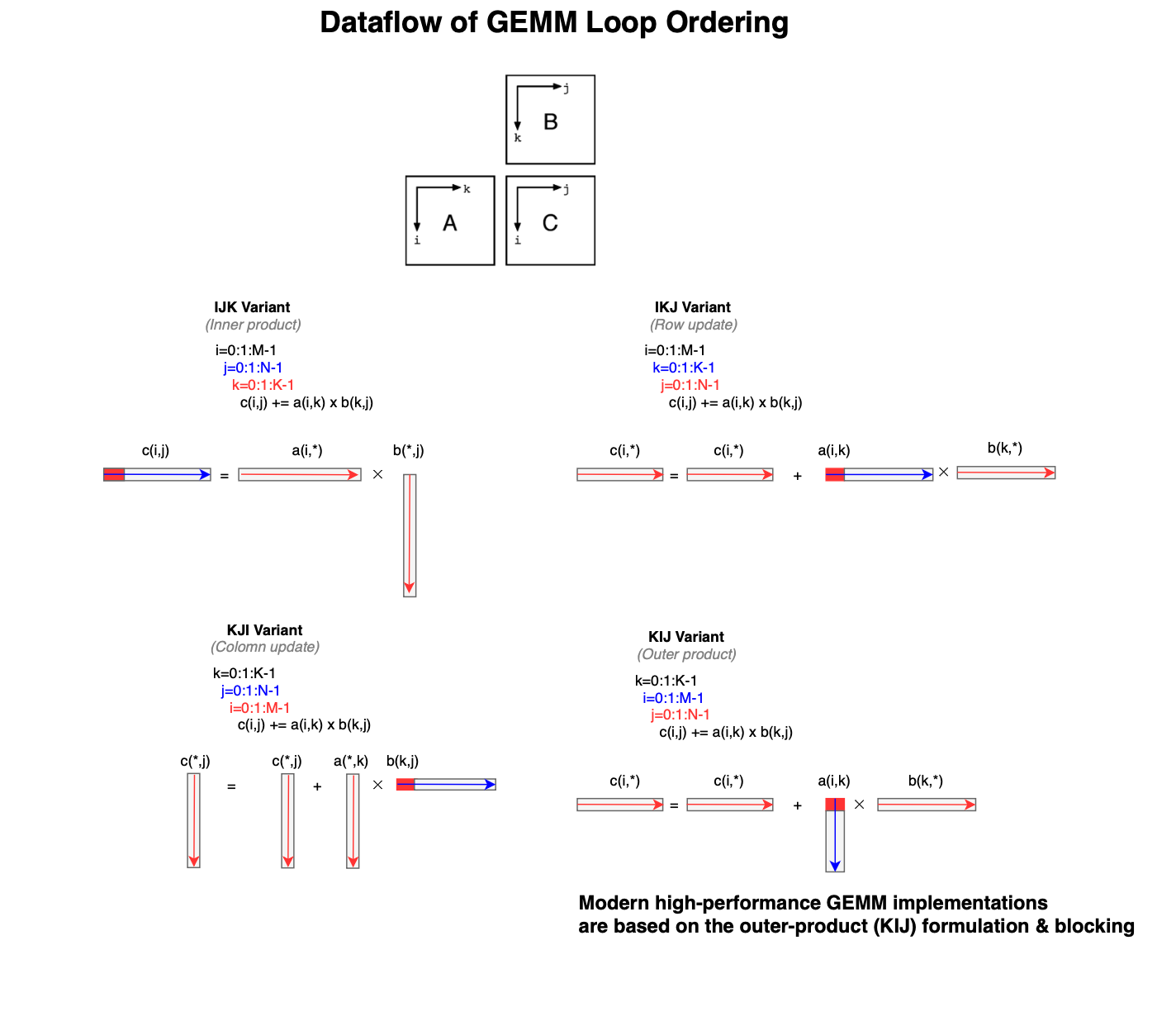

General Matrix Multiplication (GEMM)

Matrix multiplication, or GEMM, involves two matrix operands \(A \in \mathbb{R}^{M\times K}\) and \(B \in \mathbb{R}^{K\times N}\), and produces an output matrix \(C \in \mathbb{R}^{M\times N}\) given by \(C = AB\). In its simplest form, matrix multiplication involves a straightforward three-nested loop, where the innermost loop performs a scalar product. If we write \(A\) and \(B\) as \[ A = \begin{pmatrix} a_0^{t} \\ a_1^{t} \\ \vdots \\ a_{M-1}^{t} \end{pmatrix}, \qquad a_i \in \mathbb{R}^{K}, \] and \[ B = (\, b_0 \; b_1 \; \cdots \; b_{N-1} \,), \qquad b_j \in \mathbb{R}^{K}, \] then each entry of \(C\) is an inner product: \[ \underbrace{C}_{M\times N} = \underbrace{A}_{\in \mathbb{R}^{M\times K}} \underbrace{B}_{\in \mathbb{R}^{K\times N}} = \begin{pmatrix} \langle a_0, b_0 \rangle & \langle a_0, b_1 \rangle & \cdots & \langle a_0, b_{N-1} \rangle \\ \langle a_1, b_0 \rangle & \langle a_1, b_1 \rangle & \cdots & \langle a_1, b_{N-1} \rangle \\ \vdots & \vdots & \ddots & \vdots \\ \langle a_{M-1}, b_0 \rangle & \langle a_{M-1}, b_1 \rangle & \cdots & \langle a_{M-1}, b_{N-1} \rangle \end{pmatrix}. \] Each inner product \(\langle a_i , b_j \rangle\) requires K multiplications and K − 1 summations i.e 2K-1 flops. Since there are \(MN\) entries, vanilla or naive matrix multiplication costs \((2K-1)MN\) flops or for large K \(2KMN\) flops, if \(M=N=K\) we obtain \(2N^3\) flops for large N.

Implementations of GEMM exist in different flavors, obtained by permuting the order of the loops (six variants in total [15,16]) and corresponding to three different dataflows (i.e., how data is accessed). All variants require \(2MNK\) floating-point operations (flops). The \(ijk\) variant is the most straightforward, for fixed \(i\) and \(j\), it computes the scalar product by iterating over the \(K\) dimension. On the other hand, the \(ikj\) and \(kij\) variants compute partial sums while iterating over the \(N\) dimension. In the \(ikj\) variant, once the \(K\) dimension has been traversed, one row of \(C\) is fully computed, resulting in row-oriented updates. In contrast, the \(kji\) variant places the traversal of the \(K\) dimension in the outermost loop and \(i\) in the innermost loop, yielding column-oriented updates. While any of the aforementioned versions or variants produces a correct result, the data access pattern can significantly influence performance due to hardware effects (e.g., cache misses); particularly pronounced for large matrices. Instead of \(C = AB\) we ususally consider \( C = AB + C\) i,e \[ \underbrace{C}_{M\times N} = \begin{pmatrix} \langle a_0, b_0 \rangle + c_{00} & \langle a_0, b_1 \rangle + c_{01} & \cdots & \langle a_0, b_{N-1} \rangle + c_{0,N-1} \\ \langle a_1, b_0 \rangle + c_{10} & \langle a_1, b_1 \rangle + c_{11} & \cdots & \langle a_1, b_{N-1} \rangle + c_{1,N-1} \\ \vdots & \vdots & \ddots & \vdots \\ \langle a_{M-1}, b_0 \rangle + c_{M-1,0} & \langle a_{M-1}, b_1 \rangle + c_{M-1,1} & \cdots & \langle a_{M-1}, b_{N-1} \rangle + c_{M-1,N-1} \end{pmatrix}. \] Each \(\langle a_{i}, b_j \rangle + c_{i,j}\) requires requires K FMAs and hence 2K flops. Overall AB + C requires 2KMN flops.

For later discussions, we need to get comfortable with partitioning matrices. We introduce some background on matrix partitioning [17,18]. Consider matrices \(A \in \mathbb{R}^{M\times K}\), \(B \in \mathbb{R}^{K\times N}\), and \[ C := AB + C, \] where \(C \in \mathbb{R}^{M\times N}\). Following similar notation presented in [17,18], matrix \(A\) (and similarly for the other matrices) can be partitioned either horizontally or vertically: \[ A = (A_0 \; | \; \cdots \; | \; A_{n-1}) = \begin{pmatrix} \hat{A}_0 \\ \vdots \\ \hat{A}_{m-1} \end{pmatrix}. \] We will use these partitionings extensively in the register blocking section. Picking one dimension for partitioning [17,18] leads to different ways of computing \(C\). If the partitioning happens along the \(N\) dimension, i.e., \(C\) and \(B\) are sliced vertically, then multiple matrix–panel multiplications are used to compute \(C\), that is, \[ C_j = AB_j + C_j \qquad \text{for all } j = 0,\ldots,n-1. \] Equivalently, \[ C = (C_0 \; | \; \cdots \; | \; C_{n-1}) := AB + C = A(B_0 \; | \; \cdots \; | \; B_{n-1}) + C = (AB_0 + C_0 \; | \; \cdots \; | \; AB_{n-1} + C_{n-1}). \] If one picks the \(K\) dimension, i.e., \(A\) is sliced vertically and \(B\) horizontally, we obtain a panel–panel multiplication: \[ C := AB + C = (A_0 \; | \; \cdots \; | \; A_{k-1}) \begin{pmatrix} \hat{B}_0 \\ \vdots \\ \hat{B}_{k-1} \end{pmatrix} + C = \sum_p A_p \hat{B}_p + C. \] Finally, if one picks the \(M\) dimension, i.e., \(C\) and \(A\) are sliced horizontally, then \[ C_i = \hat{A}_i B + C_i, \] which corresponds to a panel–matrix multiplication. That is, \[ C := \begin{pmatrix} \hat{A}_0 \\ \vdots \\ \hat{A}_{m-1} \end{pmatrix} B + C = \begin{pmatrix} \hat{A}_0 B + \hat{C}_0 \\ \vdots \\ \hat{A}_{m-1} B + \hat{C}_{m-1} \end{pmatrix}. \] A naive GEMM is implemented using a loop nest corresponding to an iteration space of dimension=3. There are \(3! = 6\) possible permutations (variants), each generating a different iteration order, namely \(ijk\), \(ikj\), \(kij\), \(kji\), \(jik\), and \(jki\). These six variants map to distinct data flows and memory access patterns. In particular, four different formulations can be identified: the inner-product formulation, the outer-product formulation, the row-wise update formulation, and the column-wise update formulation. Outer product enjoys a higher compute-to-memory ratio. For the \(ijk/jik\) variants, which are the most straightforward ones, each row of operand \(A\) is combined with each column of \(B\) to produce a scalar element of the output matrix \(C\). This corresponds to the inner-product formulation: \[ c_{m,n} = \sum_{k=1}^{K} \underbrace{a_{m,k}}_{\in \mathbb{R}} \underbrace{b_{k,n}}_{\in \mathbb{R}} . \] In the \(ikj\) variant, once the \(K\) dimension has been traversed, one row of \(C\) is fully computed, resulting in row-oriented updates: \[ C_{m,:} = \sum_{k=1}^{K} \underbrace{a_{m,k}}_{\in \mathbb{R}} \underbrace{B_{k,:}}_{\in \mathbb{R}^{1 \times N}} . \] The \(kij\) variant corresponds to the outer-product formulation, i.e. \[ C = \sum_{k=1}^{K} \underbrace{A_{:,k}}_{\in \mathbb{R}^{M \times 1}} \underbrace{B_{k,:}}_{\in \mathbb{R}^{1 \times N}} . \] The \(kji/jki\) variants place the traversal of the \(K\) dimension and the \(N\) dimension, respectively, in the outer loops and \(i\) in the innermost loop, yielding column-oriented updates: \[ C_{:,n} = \sum_{k=1}^{K} \underbrace{A_{:,k}}_{\in \mathbb{R}^{M \times 1}} \underbrace{b_{k,n}}_{\in \mathbb{R}} . \]

We look at the variant ijk and analyse its memory traffic.

For i=0:1:M-1
  For j=0:1:N-1
    For k=0:1:K-1
        c_ij += a_ik b_kj

The implementation in c is listed below:

void matmul_naive_ijk(const double *A, const double *B, double *C, int64_t n) {
    for (int i = 0; i < n; i++)
        for (int j = 0; j < n; j++) {
            for (int k = 0; k < n; k++)
                C[i * n + j] += A[i * n + k] * B[k * n + j];
        }
}

If we inspect the produced assembly code, there is only one early load of c reused during the entire k loop, A and B references are loaded and one FMA instruction is used i.e 2 FLOPS per cycle instead of one multiply followed by one add. However, the compiler did not unroll the loop nor used vector hardware, and 2 flops per iteration means very low operational intensity.

ldr     d0, [x2, x14, lsl #3]
mov     x15, x12
ldr     d1, [x0, x13, lsl #3]
ldr     d2, [x15]
fmadd   d0, d1, d2, d0

Looking at the figure below, the performance gap between openblas (1 core) and our custom implementation is huge. We will focusing on shrinking this gap in the rest of this post. But first lets understand why is the performance is terrible.

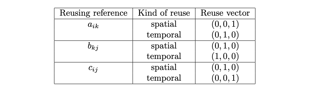
Suppose that N,M and K are very large. The reuse vectors for each reference are listed below. Temporal reuse means a reference accesses the same data element in different iterations of the loop, while spatial reuse means a reference accesses the same memory or cache line in different iterations of the loop.

The \(ijk\) loop is basically a loop nest of depth \(3\), and each iteration execution \((i,j,k)\) can be represented by an iteration vector. The first dimension corresponds to the outermost loop and the last dimension corresponds to the innermost loop. In this case the set of iteration points or nodes forms what is known as the iteration space. More generally, given a loop nest of depth \(n\), the iteration space \(I_s\) is a convex subset of \(\mathbb{Z}^n\) and is defined formally by the loop iterator variables (observe that the iteration space is a polyhedron in \(\mathbb{Z}^n\)): \[ I_s = \left\{ \vec{i} = \begin{pmatrix} i_1 \\ \vdots \\ i_n \end{pmatrix} \;\middle|\; \ell_p \le i_p \le u_p , \quad \forall p = 1 \dots n \right\} \] \(\vec{i}\) represents a single iteration of the \(n\)-deep loop nest. \(\ell_p\) and \(u_p\) are the lower and upper bounds of \(i_p\). If iteration \(i\) executes after iteration \(j\), then one says that \(j\) is lexicographically greater than \(i\). The iteration space is also said to be a polytope because the polyhedron is bounded by the loop bounds. Before we see if we can apply a loop transformation to reduce data traffic and thus increase arithmetic intensity (and thereby performance), let us compute the capacity misses (ignoring conflict misses which will be discussed later, and assuming an optimal cache policy). \(A\) will generate \(MKN/b\) misses where \(b\) is the number of elements a cache line can host. For \(B\) the number of misses is \(MNK\) because \(B\) is accessed in column order while being stored using row-major layout. Finally \(C\) will generate \(MN/b\) cache misses. If \(M=N=K\) then the total capacity misses are \[ N^3 + \frac{N^3}{b} + \frac{N^2}{b} \] which is equivalent to \[ N^3\left(1 + \frac{1}{b}\right) \] for large \(N\). Now we can fix the problem of poor access to \(B\) by permuting the loops, i.e.\ from \(ijk\) to \(ikj\). But first we must understand why the loop interchange in this case is valid, i.e. that we are not going to break data flow or dependences and thus destroy program semantics. Before applying any loop transformation, we must ensure that data dependences are preserved. If an iteration \(i_1\) writes to a memory location and \(i_2\) reads that memory location, then both \(i_1\) and \(i_2\) are dependent and \(i_2 - i_1\) is the dependence distance vector. There are three types of dependencies,true dependence (write followed by a read), output dependence (two writes to the same location) and anti-dependence (a read followed by a write). There is also read-after-read dependence, but it does not matter because the order of reads does not affect correctness. To determine dependences, we can represent iteration points as nodes in a convex polyhedron (i.e. the iteration space) and draw arrows from one point to another to represent dependences.
Loop interchange is not always legal (legal here meaning that program semantics are preserved), because it reorders computation. If we represent a loop transformation as a unimodular matrix transformation operating on the iteration space, then a transformation is legal if in the original space every iteration \(\vec{i}\) that must happen before \(\vec{j}\) is still preserved after transformation (i.e.\ original data dependences are preserved). If \[ \vec{j} = \vec{i} + \vec{d} \] where \(\vec{d} = \vec{j}-\vec{i}\) is the distance vector and \(\vec{d}\) is lexicographically positive, then \(Td\) must also be lexicographically positive where \(T\) is the unimodular transformation. If \(Td\) becomes negative then it means an anti-dependence was introduced (in the same way anti-dependences can become true dependences). In the \(ijk\) variant, the only dependence vector is \((0,0,1)\) since iteration \((i,j,k)\) writes to \(c_{ij}\) and iteration \((i,j,k+1)\) reads the same location. A loop interchange such as \(ikj\) transforms the iteration space as follows: \[ T(i,j,k) = \begin{pmatrix} 1&0&0\\ 0&0&1\\ 0&1&0 \end{pmatrix} \begin{pmatrix} i\\ j\\ k \end{pmatrix} = \begin{pmatrix} i\\ k\\ j \end{pmatrix} \] Thus \[ d' = T d = \begin{pmatrix} 1&0&0\\ 0&0&1\\ 0&1&0 \end{pmatrix} \begin{pmatrix} 0\\ 0\\ 1 \end{pmatrix} = \begin{pmatrix} 0\\ 1\\ 0 \end{pmatrix} \] The resulting distance vector is still lexicographically positive and therefore the transformation is valid. In other words, transformed dependence vectors must not point backward in the new iteration space. For example, transforming a direction vector from \((+, -)\) to \((-, +)\) is illegal. If a transformation creates an illegal dependence, then loop interchange is not legal. Now that we understand that we can interchange loops, let us discuss the \(ikj\) variant where the iteration space is transformed:

 For i=0:1:M-1
   For k=0:1:K-1
      For j=0:1:N-1
        c_ij += a_ik b_kj

The c code is listed below:

void matmul_ikj(const double *restrict A, const double *restrict B, double *restrict C, int64_t n) {
    for (int i = 0; i < n; i++)
        for (int k = 0; k < n; k++)
            for (int j = 0; j < n; j++)
                C[i * n + j] += A[i * n + k] * B[k * n + j];
}

Inspecting the produced assembly code, thanks to the loop interchange transformation, the compiler was capable of applying a loop unrolling and thereby reducing loop overhead in addition to reducing cache misses. Additionally, the compiler used vector instructions as listed below (fmla.2d is a vector fma ).

ldp     q2, q3, [x5, #-32]
ldp     q4, q5, [x5], #64
ldp     q6, q7, [x4, #-32]
ldp     q16, q17, [x4]
fmla.2d v6, v2, v1
fmla.2d v7, v3, v1
fmla.2d v16, v4, v1
fmla.2d v17, v5, v1

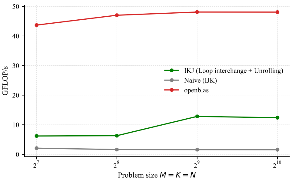
So now with the loop interchange we unlocked loop unrolling and also the use of vectorization which leads to higher arithmetic intensity and this better performance. This can be confirmed below. We still have some gap to bridge but we will work on it.

Even though the \(ikj\) variant reduces capacity misses, we can further increase arithmetic intensity using tiling (blocking). Tiling consists of strip-mining followed by loop permutation and turns a \(3\)-loop nest into a loop nest of depth \(4\), \(5\), or \(6\). If one or more inner loops carry reuse (e.g the loop k carry reuse in the \(ijk\) variant because \(c_{ij}\) is reused across many iterations of the k loop) and they can be interchanged, then the loops would be tiled. Suppose we use one-level tiling. We strip-mine the \(j\) loop and permute it, resulting in panels of \(B\) of size \(K \times n_c\). \[ C_j = A B_j \]

For jj=0:n_c:N-n_c-1
   For i=0:1:M-1
      For k=0:1:K-1
         For j=jj:1:jj+n_c-1
            c_ij += a_ik b_kj

The working set of the innermost loop is then reduced to \[ MK + Kn_c + Mn_c \] Now consider two-level tiling. We strip-mine the \(i\) loop and permute it, producing panels of \(C\) of size \(m_c \times n_c\). \[ \hat{C}_i^j = \hat{A}_i B_j \]

For ii=0:m_c:M-m_c-1
  For jj=0:n_c:N-n_c-1
     For i=ii:1:ii+m_c-1
        For k=0:1:K-1
           For j=jj:1:jj+n_c-1
              c_ij += a_ik b_kj

The working set becomes \[ m_cn_c + m_cK + Kn_c \] Finally consider three-level tiling. We strip-mine the \(k\) loop and permute it, producing panels of \(A\) of size \(m_c \times k_c\). \[ C^{j\hat{i}} = \sum_k \hat{A}^{i}_k \hat{B}^{j}_k \]

For ii=0:m_c:M-m_c-1
   For kk=0:k_c:K-k_c-1
      For jj=0:n_c:N-n_c-1
         For i=ii:1:ii+m_c-1
            For k=kk:1:kk+k_c-1
               For j=jj:1:jj+n_c-1
                  c_ij += a_ik b_kj

The working set becomes \[ m_cn_c + m_ck_c + k_cn_c \] Suppose we choose parameters \(m_c, k_c, n_c\) so that \[ m_cn_c + m_ck_c + k_cn_c \] fits in cache. The total cache misses then become: \[ A : MK/b \] \[ B : \frac{MKN}{bm_c} \] \[ C : \frac{MKN}{k_cb} \] If \(M=N=K\) and \(m_c=k_c=n_c=E\): \[ 2\frac{N^3}{bE} + \frac{N^2}{b} \] which is approximately \[ \frac{2N^3}{bE} \] Thus \[ CM(ikj_{\text{tiled}}) = E \cdot CM(ikj) \] i.e. tiling reduces cache misses by a factor of \(E\). We can improve further using register tiling (multi-level tiling) to reduce load/store instructions, enable register reuse, and expose more instruction-level parallelism (ILP). To implement multi-level tiling (i.e., to combine register-level and cache-level tiling), one level of tiling is performed by repeatedly applying the strip-mining and loop permutation transformations. In this case, a first level of tiling produces tiles of \(A\), \(B\), and \(C\) of size \(m_c \times k_c\), \(k_c \times n_c\), and \(m_c \times n_c\), respectively. These tiles then undergo another level of tiling to produce micro-tiles of \(A_{m_c \times k_c}\), \(B_{k_c \times n_c}\), and \(C_{m_c \times n_c}\) of size \(m_r \times k_r\), \(k_r \times n_r\), and \(m_r \times n_r\). Usually, the micro-tile parameters are chosen so that \[ m_r n_r + n_r + m_r \] fits in the vector registers, enabling the implementation of rank-1 updates using the outer product formulation. In other words, the matrix multiplication of the micro-tiles (called the micro-kernel) uses an outer-product data flow where the \(C\) micro-tile is resident in registers while one column of micro tile \(A\) and one row of micro tile \(B\) are hosted in registers. Additionally, regarding cache tiling, the tile \(A_{m_c \times k_c}\) is reused across the \(jjj\) loop, so the configuration is chosen such that it can be hosted in the L3 cache. Next, \(B_{k_c \times n_c}\) is reused across the \(ii\) loop, so it should reside in the L2 cache. Finally, the micro-panel \(A_{m_r \times k_r}\) is reused across the \(jj\) loop, so we keep it in the L1 cache. A straightforward multi-level tiled implementation can be written as:

For iii=0:m_c:M-1
   For kkk=0:k_c:K-1
      For jjj=0:n_c:N-1
         For ii=iii:m_r:iii+m_c-1
            For kk=kkk:k_r:kkk+k_c-1
               For jj=jjj:n_r:jjj+n_c-1
                  For k=kk:1:kk+k_r-1
                     For i=ii:1:ii+m_r-1
                        For j=jj:1:jj+n_r-1
                            C[i,j] += A[i,k] * B[k,j]

Instead of the above formulation, the \(K\) dimension usually undergoes only one level of strip-mining (e.g., in GotoBLAS, BLIS, and OpenBLAS), i.e., five nested loops surround the micro-kernel. In this case, the micro-kernel comprises an inner loop (labeled as LR below) that repeatedly updates an \(m_r \times n_r\) micro-tile of \(C\), denoted \(C_r\), through a sequence of \(k_c\) rank-1 updates. Each update involves a column of \(A_c\) of length \(m_r\) and a row of \(B_c\) of length \(n_r\).

For iii = 0 : m_c : M-1
   For kkk = 0 : k_c : K-1
      For jjj = 0 : n_c : N-1
      // macro kernel 
         For ii = iii : m_r : iii + m_c - 1
            For jj = jjj : n_r : jjj + n_c - 1
               # LR : micro-kernel operating on C_r (m_r × n_r)
               For k = kkk : 1 : kkk + k_c - 1
                  For i = ii : 1 : ii + m_r - 1
                     For j = jj : 1 : jj + n_r - 1
                        C[i,j] += A[i,k] * B[k,j]

or equivalently represented as:

For iii = 0 : m_c : M-1
   For kk = 0 : k_c : K-1
      For jjj = 0 : n_c : N-1
         For ii = iii : m_r : iii + m_c - 1
            For jj = jjj : n_r : jjj + n_c - 1
               # LR : micro-kernel operating on C_r (m_r × n_r)
               For k = kk : 1 : kk + k_c - 1
                  C[ii:ii+m_r-1, jj:jj+n_r-1] +=
                      A[ii:ii+m_r-1, k] * B[k, jj:jj+n_r-1]

Finally, introducing packing of the cache-level panels in order to enforce in-stride load access when used to update a micro-tile of C inside the micro-kernel yields (\(A_c\) and \(B_c\) are also aligned to cache lines boundaries, observe that \(B_c\) is packed in Loop 3 after \(A_c\) has been packed in Loop 2, the elements of \(B_c\) will likely be higher up in the memory hierarchy closer to the register file than those of \(A_c\)):

For iii = 0 : m_c : M-1
   For kkk = 0 : k_c : K-1

      // Pack A_c (m_c × k_c)
      Ac = A[iii:iii+m_c-1 , kkk:kkk+k_c-1]

      For jjj = 0 : n_c : N-1

         // Pack B_c (k_c × n_c)
         Bc = B[kkk:kkk+k_c-1 , jjj:jjj+n_c-1]

         For ii = iii : m_r : iii + m_c - 1
            For jj = jjj : n_r : jjj + n_c - 1

               # LR : micro-kernel operating on C_r (m_r × n_r)
               For k = 0 : 1 : k_c - 1
                  C[ii:ii+m_r-1, jj:jj+n_r-1] +=
                     Ac[ii-iii:ii-iii+m_r-1, k] *
                     Bc[k, jj-jjj:jj-jjj+n_r-1]

or if you will

For iii = 0 : m_c : M-1
   For kkk = 0 : k_c : K-1
      // Pack A_c (m_c × k_c)
      Ac = A[iii:iii+m_c-1 , kkk:kkk+k_c-1]

      For jjj = 0 : n_c : N-1
         // Pack B_c (k_c × n_c)
         Bc = B[kkk:kkk+k_c-1 , jjj:jjj+n_c-1]

         For ii = 0 : m_r : m_c - 1
            For jj = 0 : n_r : n_c - 1
               # LR : micro-kernel operating on C_r (m_r × n_r)
               For k = 0 : 1 : k_c - 1
                  C[iii+ii:iii+ii+m_r-1, jjj+jj:jjj+jj+n_r-1] +=
                     Ac[ii:ii+m_r-1, k] *
                     Bc[k, jj:jj+n_r-1]

Combining register tiling and cache tiling yields very good performance, as it reduces capacity cache misses, improves ILP, enables register reuse, and reduces the number of load/store operations. Observe that by shrinking the number of memory accesses, the program becomes closer to being cpu-bound rather than memory-bound, i.e., it increases the arithmetic intensity. To reduce conflict misses (and TLB misses), before invoking the micro-kernel, the \(A\) and \(B\) tiles (of dimensions \(m_c \times k_c\) and \(k_c \times n_c\), respectively) are packed into contiguous buffers. By ensuring that these packed buffers are highly reused during the computation, the cost of copying can be amortized. The packing follows the memory layout required by the architecture-dependent micro-kernel, that is in our case, \(A\) is stored in column-major form (by transposing it) and \(B\) in row-major form.

Example code for register and cache tiling are listed below:

void matmul_register_tiling(const double *__restrict A,
                            const double *__restrict B,
                            double *__restrict C,
                            int64_t n) {
    for (int64_t ii = 0; ii < n; ii += 2) {
        for (int64_t jj = 0; jj < n; jj += 2) {

            double c00 = C[(ii + 0) * n + (jj + 0)];
            double c01 = C[(ii + 0) * n + (jj + 1)];
            double c10 = C[(ii + 1) * n + (jj + 0)];
            double c11 = C[(ii + 1) * n + (jj + 1)];

            for (int64_t k = 0; k < n; ++k) {
                double a0 = A[(ii + 0) * n + k];
                double a1 = A[(ii + 1) * n + k];

                double b0 = B[k * n + (jj + 0)];
                double b1 = B[k * n + (jj + 1)];

                c00 += a0 * b0;
                c01 += a0 * b1;
                c10 += a1 * b0;
                c11 += a1 * b1;
            }

            C[(ii + 0) * n + (jj + 0)] = c00;
            C[(ii + 0) * n + (jj + 1)] = c01;
            C[(ii + 1) * n + (jj + 0)] = c10;
            C[(ii + 1) * n + (jj + 1)] = c11;
        }
    }
}

void matmul_cache_tiling(const double *restrict A, const double *restrict B, double *restrict C, int64_t n) {
    const int bs = 32;
    for (int ii = 0; ii < n; ii += bs) {
        for (int kk = 0; kk < n; kk += bs) {
            for (int i = ii; i < ii + bs; i++) {
                for (int k = kk; k < kk + bs; k++) {
                    double aik = A[i * n + k];
                    for (int j = 0; j < n; j++) {
                        C[i * n + j] += aik * B[k * n + j];
                    }
                }
            }
        }
    }
}

A naive combination of cache and register tiling would look like this:

void matmul_cache_and_register_tiling(
        const double *restrict A,
        const double *restrict B,
        double *restrict C,
        int64_t n)
{
    const int64_t bs = 32;
    for (int64_t iii = 0; iii < n; iii += bs) {
        for (int64_t kkk = 0; kkk < n; kkk += bs) {
            for (int64_t jjj = 0; jjj < n; jjj += bs) {

                for (int64_t ii = iii; ii < iii + bs; ii += 4) {
                    for (int64_t jj = jjj; jj < jjj + bs; jj += 4) {

                        double c00 = C[(ii + 0) * n + (jj + 0)];
                        double c01 = C[(ii + 0) * n + (jj + 1)];
                        double c02 = C[(ii + 0) * n + (jj + 2)];
                        double c03 = C[(ii + 0) * n + (jj + 3)];

                        double c10 = C[(ii + 1) * n + (jj + 0)];
                        double c11 = C[(ii + 1) * n + (jj + 1)];
                        double c12 = C[(ii + 1) * n + (jj + 2)];
                        double c13 = C[(ii + 1) * n + (jj + 3)];

                        double c20 = C[(ii + 2) * n + (jj + 0)];
                        double c21 = C[(ii + 2) * n + (jj + 1)];
                        double c22 = C[(ii + 2) * n + (jj + 2)];
                        double c23 = C[(ii + 2) * n + (jj + 3)];

                        double c30 = C[(ii + 3) * n + (jj + 0)];
                        double c31 = C[(ii + 3) * n + (jj + 1)];
                        double c32 = C[(ii + 3) * n + (jj + 2)];
                        double c33 = C[(ii + 3) * n + (jj + 3)];

                        for (int64_t k = kkk; k < kkk + bs; ++k) {

                            double a0 = A[(ii + 0) * n + k];
                            double a1 = A[(ii + 1) * n + k];
                            double a2 = A[(ii + 2) * n + k];
                            double a3 = A[(ii + 3) * n + k];

                            double b0 = B[k * n + (jj + 0)];
                            double b1 = B[k * n + (jj + 1)];
                            double b2 = B[k * n + (jj + 2)];
                            double b3 = B[k * n + (jj + 3)];

                            c00 += a0 * b0;
                            c01 += a0 * b1;
                            c02 += a0 * b2;
                            c03 += a0 * b3;

                            c10 += a1 * b0;
                            c11 += a1 * b1;
                            c12 += a1 * b2;
                            c13 += a1 * b3;

                            c20 += a2 * b0;
                            c21 += a2 * b1;
                            c22 += a2 * b2;
                            c23 += a2 * b3;

                            c30 += a3 * b0;
                            c31 += a3 * b1;
                            c32 += a3 * b2;
                            c33 += a3 * b3;
                        }

                        C[(ii + 0) * n + (jj + 0)] = c00;
                        C[(ii + 0) * n + (jj + 1)] = c01;
                        C[(ii + 0) * n + (jj + 2)] = c02;
                        C[(ii + 0) * n + (jj + 3)] = c03;

                        C[(ii + 1) * n + (jj + 0)] = c10;
                        C[(ii + 1) * n + (jj + 1)] = c11;
                        C[(ii + 1) * n + (jj + 2)] = c12;
                        C[(ii + 1) * n + (jj + 3)] = c13;

                        C[(ii + 2) * n + (jj + 0)] = c20;
                        C[(ii + 2) * n + (jj + 1)] = c21;
                        C[(ii + 2) * n + (jj + 2)] = c22;
                        C[(ii + 2) * n + (jj + 3)] = c23;

                        C[(ii + 3) * n + (jj + 0)] = c30;
                        C[(ii + 3) * n + (jj + 1)] = c31;
                        C[(ii + 3) * n + (jj + 2)] = c32;
                        C[(ii + 3) * n + (jj + 3)] = c33;
                    }
                }
            }
        }
    }
}

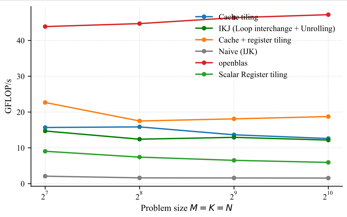
If we look at the performance, we have closed a bit the gap but we are still far behind openblas; yes I was desperate at some point but we don't give up and lets see how to can we get close to openblas by writing a code that looks close to high computational kernels.

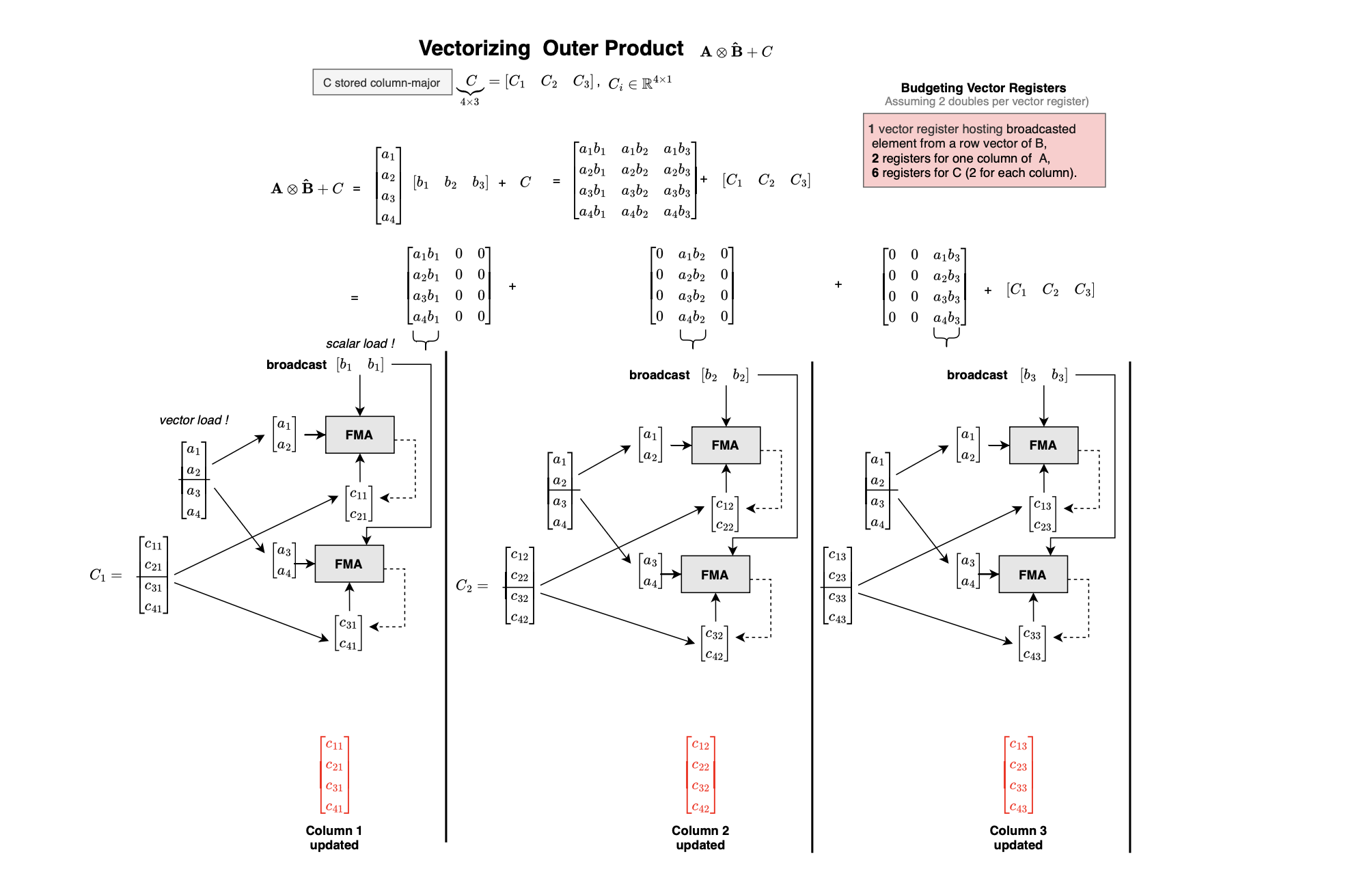
Most high-performance code is written using in-lined assembly code (e.g openblas or blis microkernel) or using vector intrinsic functions that enable access the vector instructions and vector registers within the c programming language. The microkernel code is listed below.

void matmul_micro_kernel_4x8(
        const double *restrict A,
        const double *restrict B,
        double *restrict C,
        int64_t n)
{
    const int64_t m_c = 64, n_c = 64, k_c = 64;// this can be determined using analytic or empirical approach
    // it is assumed that n is larger thatn 64 and power of two

#pragma omp parallel
    {
        size_t size_Ac = m_c * k_c;
        size_t size_Bc = k_c * n_c;
        size_t pad = 8;
        double *base = NULL;
        posix_memalign((void**)&base, 64,
                       (size_Ac + size_Bc + pad) * sizeof(double));
        double *A_c = base;
        double *B_c = base + size_Ac + pad;

#pragma omp for schedule(static)
        for (int64_t iii = 0; iii < n; iii += m_c) {
            for (int64_t kkk = 0; kkk < n; kkk += k_c) {

                // we pack A_c by column and A is originally stored using row major layout
                // this maps to  Ac = A(iii:iii+mc-1, kkk:kkk+kc-1)
                // i.e Ac(0,0) = A(iii,kkk) = A[iii*n + kkk]
                // and thus Ac(k,i) = A(iii + i,kkk+k) = A[(iii+i)*n + kkk+k] and this explains the code below
                for (int64_t k = 0 ; k < k_c; ++k) {
                    for (int64_t i = 0; i < m_c; ++i) {
                        A_c[k * m_c + i] = A[(iii + i) * n + (kkk + k)];
                    }
                }

                for (int64_t jjj = 0; jjj < n; jjj += n_c) {

                    // B is already stored using row major layout so we merely just copy the block
                    // Bc(k,j) = B(kkk+k,jjj+j) = B[(kkk+k)*n + jjj+j]
                    for (int64_t k = 0; k < k_c; ++k) {
                        for (int64_t j = 0; j < n_c; ++j) {
                            B_c[k * n_c + j] = B[(kkk + k) * n + (jjj + j)];
                        }
                    }

                    for (int64_t ii = iii; ii < iii + m_c; ii += 4) {
                        for (int64_t jj = jjj; jj < jjj + n_c; jj += 8) {

                            // as explained micro tile C is resident so we load the 4x8 micro tile
                            // for each row we need 4 registers i.e one register for each two consecutive elements
                            // and we use axpy ops on the rows not colomns
                            // because C is stored using row major layout

                            // below is one row (c00 is first row and c00_i is block if row 0)
                            float64x2_t c00_0 = vld1q_f64(&C[(ii+0)*n + jj + 0]);
                            float64x2_t c00_1 = vld1q_f64(&C[(ii+0)*n + jj + 2]);
                            float64x2_t c01_0 = vld1q_f64(&C[(ii+0)*n + jj + 4]);
                            float64x2_t c01_1 = vld1q_f64(&C[(ii+0)*n + jj + 6]);

                            float64x2_t c10_0 = vld1q_f64(&C[(ii+1)*n + jj + 0]);
                            float64x2_t c10_1 = vld1q_f64(&C[(ii+1)*n + jj + 2]);
                            float64x2_t c11_0 = vld1q_f64(&C[(ii+1)*n + jj + 4]);
                            float64x2_t c11_1 = vld1q_f64(&C[(ii+1)*n + jj + 6]);

                            float64x2_t c20_0 = vld1q_f64(&C[(ii+2)*n + jj + 0]);
                            float64x2_t c20_1 = vld1q_f64(&C[(ii+2)*n + jj + 2]);
                            float64x2_t c21_0 = vld1q_f64(&C[(ii+2)*n + jj + 4]);
                            float64x2_t c21_1 = vld1q_f64(&C[(ii+2)*n + jj + 6]);

                            float64x2_t c30_0 = vld1q_f64(&C[(ii+3)*n + jj + 0]);
                            float64x2_t c30_1 = vld1q_f64(&C[(ii+3)*n + jj + 2]);
                            float64x2_t c31_0 = vld1q_f64(&C[(ii+3)*n + jj + 4]);
                            float64x2_t c31_1 = vld1q_f64(&C[(ii+3)*n + jj + 6]);

                            // now that all the micro tiles are loaded in vector registers
                            // we start doing rank-1 updates for all
                            // I use unrolling with factor 2

                            for (int64_t k = 0; k < k_c; k += 2) {

                                // unroll factor k
                                //C[ii:ii+m_r-1, jj:jj+n_r-1] +=
                                //                     Ac[ii-iii:ii-iii+m_r-1, k] *
                                //                     Bc[k, jj-jjj:jj-jjj+n_r-1]
                                float64x2_t br_0 = vld1q_f64(&B_c[(k + 0) * n_c + (jj - jjj) + 0]);
                                float64x2_t br_2 = vld1q_f64(&B_c[(k + 0) * n_c + (jj - jjj) + 2]);
                                //load second part of the row of b
                                float64x2_t br_4 = vld1q_f64(&B_c[(k + 0) * n_c +  (jj - jjj) + 4]);
                                float64x2_t br_6 = vld1q_f64(&B_c[(k + 0) * n_c +  (jj - jjj) + 6]);

                                // I repeat it here for convenience
                                //C[ii:ii+m_r-1, jj:jj+n_r-1] +=
                                //                     Ac[ii-iii:ii-iii+m_r-1, k] *
                                //                     Bc[k, jj-jjj:jj-jjj+n_r-1]

                                double *ar = &A_c[(k + 0) * m_c + (ii - iii)];
                                // because C is stored using row major layout we must brodcast a and not b
                                // you can do the math to convice yourself
                                // we load one column of Ac which demands two vector registers for the 4 elements as mr =4
                                float64x2_t ar0 = vld1q_f64(ar);
                                float64x2_t ar1 = vld1q_f64(ar + 2);

                                // axpy ops
                                float64x2_t ar00 = vdupq_laneq_f64(ar0, 0);
                                c00_0 = vfmaq_f64(c00_0, ar00, br_0);
                                c00_1 = vfmaq_f64(c00_1, ar00, br_2);
                                c01_0 = vfmaq_f64(c01_0, ar00, br_4);
                                c01_1 = vfmaq_f64(c01_1, ar00, br_6);

                                float64x2_t ar01 = vdupq_laneq_f64(ar0, 1);
                                c10_0 = vfmaq_f64(c10_0, ar01, br_0);
                                c10_1 = vfmaq_f64(c10_1, ar01, br_2);
                                c11_0 = vfmaq_f64(c11_0, ar01, br_4);
                                c11_1 = vfmaq_f64(c11_1, ar01, br_6);

                                float64x2_t ar10 = vdupq_laneq_f64(ar1, 0);
                                c20_0 = vfmaq_f64(c20_0, ar10, br_0);
                                c20_1 = vfmaq_f64(c20_1, ar10, br_2);
                                c21_0 = vfmaq_f64(c21_0, ar10, br_4);
                                c21_1 = vfmaq_f64(c21_1, ar10, br_6);

                                float64x2_t ar11 = vdupq_laneq_f64(ar1, 1);
                                c30_0 = vfmaq_f64(c30_0, ar11, br_0);
                                c30_1 = vfmaq_f64(c30_1, ar11, br_2);
                                c31_0 = vfmaq_f64(c31_0, ar11, br_4);
                                c31_1 = vfmaq_f64(c31_1, ar11, br_6);

                                // now we do the same as above but for the second unroll factor k+1
                                float64x2_t br1_0 = vld1q_f64(&B_c[(k + 1) * n_c + (jj - jjj) + 0]);
                                float64x2_t br1_2 = vld1q_f64(&B_c[(k + 1) * n_c + (jj - jjj) + 2]);
                                float64x2_t br1_4 = vld1q_f64(&B_c[(k + 1) * n_c + (jj - jjj) + 4]);
                                float64x2_t br1_6 = vld1q_f64(&B_c[(k + 1) * n_c + (jj - jjj) + 6]);

                                double *ar_1 = &A_c[(k + 1) * m_c + (ii - iii)];
                                float64x2_t ar1_0 = vld1q_f64(ar_1);
                                float64x2_t ar1_2 = vld1q_f64(ar_1 + 2);

                                float64x2_t ar1_00 = vdupq_laneq_f64(ar1_0, 0);

                                c00_0 = vfmaq_f64(c00_0, ar1_00, br1_0);
                                c00_1 = vfmaq_f64(c00_1, ar1_00, br1_2);
                                c01_0 = vfmaq_f64(c01_0, ar1_00, br1_4);
                                c01_1 = vfmaq_f64(c01_1, ar1_00, br1_6);

                                float64x2_t ar1_01 = vdupq_laneq_f64(ar1_0, 1);
                                c10_0 = vfmaq_f64(c10_0, ar1_01, br1_0);
                                c10_1 = vfmaq_f64(c10_1, ar1_01, br1_2);
                                c11_0 = vfmaq_f64(c11_0, ar1_01, br1_4);
                                c11_1 = vfmaq_f64(c11_1, ar1_01, br1_6);

                                float64x2_t ar1_20 = vdupq_laneq_f64(ar1_2, 0);
                                c20_0 = vfmaq_f64(c20_0, ar1_20, br1_0);
                                c20_1 = vfmaq_f64(c20_1, ar1_20, br1_2);
                                c21_0 = vfmaq_f64(c21_0, ar1_20, br1_4);
                                c21_1 = vfmaq_f64(c21_1, ar1_20, br1_6);

                                float64x2_t ar1_21 = vdupq_laneq_f64(ar1_2, 1);
                                c30_0 = vfmaq_f64(c30_0, ar1_21, br1_0);
                                c30_1 = vfmaq_f64(c30_1, ar1_21, br1_2);
                                c31_0 = vfmaq_f64(c31_0, ar1_21, br1_4);
                                c31_1 = vfmaq_f64(c31_1, ar1_21, br1_6);
                            }

                            // after ranks updates we store the microtile C 4x8
                            vst1q_f64(&C[(ii+0)*n + jj + 0], c00_0);
                            vst1q_f64(&C[(ii+0)*n + jj + 2], c00_1);
                            vst1q_f64(&C[(ii+0)*n + jj + 4], c01_0);
                            vst1q_f64(&C[(ii+0)*n + jj + 6], c01_1);

                            vst1q_f64(&C[(ii+1)*n + jj + 0], c10_0);
                            vst1q_f64(&C[(ii+1)*n + jj + 2], c10_1);
                            vst1q_f64(&C[(ii+1)*n + jj + 4], c11_0);
                            vst1q_f64(&C[(ii+1)*n + jj + 6], c11_1);

                            vst1q_f64(&C[(ii+2)*n + jj + 0], c20_0);
                            vst1q_f64(&C[(ii+2)*n + jj + 2], c20_1);
                            vst1q_f64(&C[(ii+2)*n + jj + 4], c21_0);
                            vst1q_f64(&C[(ii+2)*n + jj + 6], c21_1);

                            vst1q_f64(&C[(ii+3)*n + jj + 0], c30_0);
                            vst1q_f64(&C[(ii+3)*n + jj + 2], c30_1);
                            vst1q_f64(&C[(ii+3)*n + jj + 4], c31_0);
                            vst1q_f64(&C[(ii+3)*n + jj + 6], c31_1);
                        }
                    }
                }
            }
        }
        free(base);
    }
}

We use vld1q_f64() and vst1q_f64() to load and store vectors of two doubles, respectively. The intrinsic vdupq_laneq_f64() is used to broadcast a selected lane across all elements of a vector, and vfmaq_f64() performs a fused multiply-add or fma operation on vectors. Before using these intrinsic functions, you must include the header file #include <arm_neon.h>. In order to reduce cache misses, A and B panels are packed using colomn and row major layout respectively.

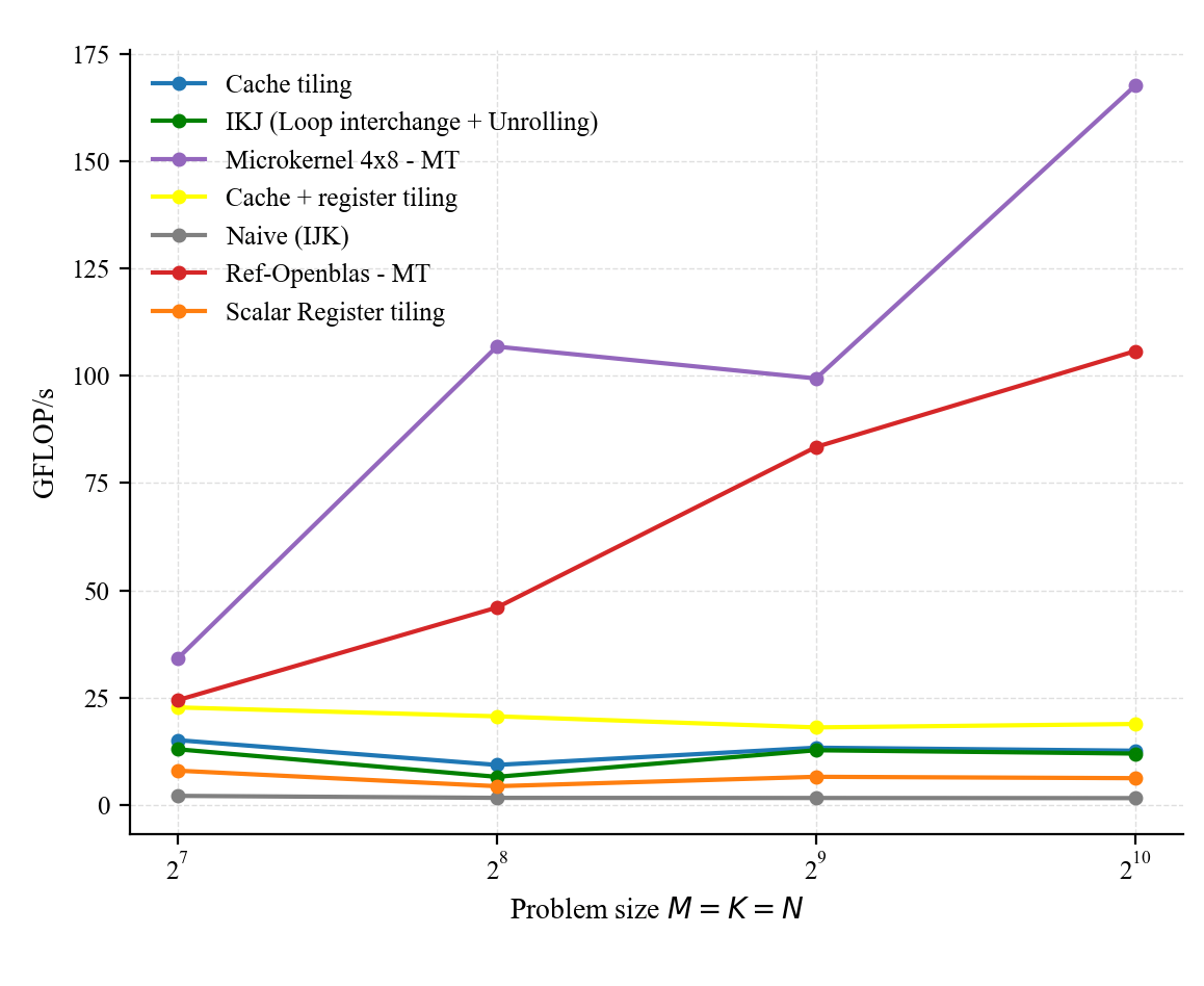
Looking at the performance plot, we have significantly closed the gap.

We can even improve further the performance using multithreading (using OpenMP for instance). The performance for both our custom micro kernel and openblas is show below (remember that our micro kernel assumes ideal sizes and comparison here is not really very fair; but again the goal is not to compete with openblas and to develop a library, instead the post aims to illustrate how fast GEMM are implemented).

GEMM Micro-Kernel Optimization

The microkernel operates on the submatrices \(A^r\), \(B^r\), and \(C^r\), where \[ A^r \in \mathbb{R}^{m_r \times k_c}, \qquad B^r \in \mathbb{R}^{k_c \times n_r}, \qquad C^r \in \mathbb{R}^{m_r \times n_r}. \] Its computation is organized as \(k_c\) rank-1 updates, following an outer-product formulation. The output block \(C^r\), which resides in registers, should be chosen to be approximately square for example, \(8 \times 6\). This is because the microkernel intensity (when \(k_c \) is large) \[ \frac{2 m_r n_r}{m_r + n_r}, \] is maximized when \(n_r = m_r\). In fact, consider \(f(x,y) = \frac{xy}{x+y}\), where \(x,y\) are defined over \(\mathbb{R}_+^2\) under the constraint \(x + y = C\) (because the vector register file is finite). Since \(f\) is concave, \(-f\) is convex, and this guarantees that a local minimum of \(-f\) is a global minimum, and thus a global maximum for \(f\). The Lagrangian is given by: \[ f(x,y) - \lambda (x + y - C), \] and the optimal point satisfies \(x = y = C/2\). Now, \(m_r\) and \(n_r\) cannot always be equal, i.e., \(C^r\) cannot always be square or said differently we cannot always have a perfectly square micro-kernel, because \(m_r\) should be a multiple of the vector register length. Since we are using \(m_r n_r + m_r + 1\)elements in the vector register file, this corresponds to \[ \frac{m_r n_r}{e} + \frac{m_r}{e} + 1 \] vector registers, where \(e\) is the number of elements that can be stored in a vector register. Therefore, choosing \(m_r = n_r\) is not always the best solution.

The microkernel computes \[ C^r \mathrel{+}= \sum_{p=1}^{k_c} A^r_p \, \hat{B}^r_p, \] where \(A^r_p\) denotes the \(p\)-th column of \(A^r\), of size \(m_r \times 1\), and \(\hat{B}^r_p\) denotes the \(p\)-th row of \(B^r\), of size \(1 \times n_r\). For each \(p\), the outer product \(A^r_p \hat{B}^r_p\) is accumulated into \(C^r\). More specifically, each column \(j\) of \(C^r\) is updated as \[ C^r_j \mathrel{+}= A^r_p \, \hat{B}^r_p(j), \] where \(\hat{B}^r_p(j)\) is a scalar broadcasted into a vector register, allowing the update to be carried out efficiently using FMA instructions. The register file must host \(m_r n_r + m_r + 1\) elements: the block \(C^r\), one column vector \(A^r_p\), and one scalar from \(\hat{B}^r_p\). All \(n_r\) column updates of \(C^r\) are typically fully unrolled, and this procedure is repeated for \(p = 1, \dots, k_c\). The reason for using the outer-product formulation at the microkernel level is that it minimizes register pressure while maximizing data reuse. Alternative loop orderings generally require more register storage. For example, a \(jik\)-style formulation would require enough register space for \(m_r k_c + k_c n_r + m_r n_r\) values in order to retain operands in registers and avoid excessive data movement. Assuming computation and data movement cannot be perfectly overlapped, an effective microkernel should maximize the fraction of time spent performing useful floating-point operations rather than moving data.

Finally, note that how the rank-1 udpates are executed, \(A^r\) should be packed in column-major order while \(B^r\) hosted using row-major form.

I did not really test prefetching but it can help a bit to overlap computation and data movement (and thus reduces the number of cycles required to perform the mult). Note however that prefetching does not increasing operational or arithmetic intensity as the blocks are still loaded in the cache (it is just when).

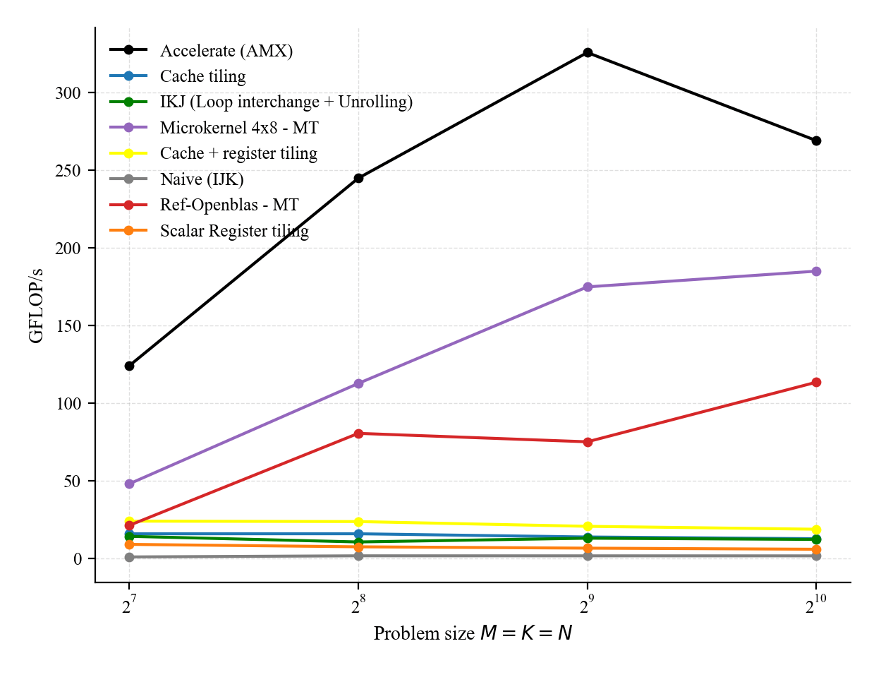
In addition to the NEON ISA, the Apple M1 supports AMX (Advanced Matrix Extensions) [6], as in other Apple Silicon M-series chips. AMX is an undocumented, specialized Apple matrix coprocessor controlled via dedicated cpu instructions, capable of accelerating matrix–matrix products (e.g., via outer-product computations) by an order of magnitude. Although not publicly documented, AMX can be utilized through the Accelerate framework’s BLAS routines, which provide highly optimized libraries. As shown below, Accelerate outperforms OpenBLAS for all FP64 matrix–matrix multiplication problem sizes. This is not a surprise, as OpenBLAS relies on 128-bit NEON instructions.

OpenBLAS Source Code Analysis

If we look at the blocking strategy used in OpenBLAS for the DGEMM routine [https://github.com/OpenMathLib/OpenBLAS/blob/develop/driver/level3/level3.c]:

void cblas_dgemm(const CBLAS_LAYOUT layout, const CBLAS_TRANSPOSE TransA,
                 const CBLAS_TRANSPOSE TransB, const int M, const int N,
                 const int K, const double alpha, const double  *A,
                 const int lda, const double  *B, const int ldb,
                 const double beta, double  *C, const int ldc)

It computes the classic GEMM operation \( C = \alpha AB + \alpha C\). The implementation begins by allocating a contiguous buffer used for packing sub-blocks of matrices A and B and reduce cache conflict misses:

 buffer = (XFLOAT *)blas_memory_alloc(0);
 #if defined(ARCH_LOONGARCH64) && !defined(NO_AFFINITY)
  sa = (XFLOAT *)((BLASLONG)buffer + (WhereAmI() & 0xf) * GEMM_OFFSET_A);
#else
  sa = (XFLOAT *)((BLASLONG)buffer + GEMM_OFFSET_A);
#endif

sb = (XFLOAT *)(((BLASLONG)sa +
        ((GEMM_P * GEMM_Q * COMPSIZE * SIZE + GEMM_ALIGN) & ~GEMM_ALIGN))
        + GEMM_OFFSET_B);

Here, sa and sb are buffers that hold packed panels of A and B, respectively. As discussed earlier, packing is critical as it ensures contiguous memory access within the compute kernel. The core computation is implemented using a blocking strategy. While the loop structure does not exactly follow the canonical GotoBLAS algorithm formulation, the same principles applies, multilevel tiling and data packing. The algorithm iterate over tiles:

 for(js = n_from; js < n_to; js += GEMM_R){
...
  for(ls = 0; ls < k; ls += min_l){
  ...
    for(is = m_from + min_i; is < m_to; is += min_i)

Packs subblocks:

ICOPY_OPERATION(..., sa);

and invoke the micro-kernel:

KERNEL_OPERATION(min_i, min_jj, min_l, (void *)&xalpha,..)

Specifically the macro-kernel delegates computation to architecture-specific micro-kernels in our case it is dgemm_kernel_8x4.S which implement rank-1 updates using vector instructions. For more details, please see the OpenBLAS kernel source: https://github.com/OpenMathLib/OpenBLAS/blob/develop/kernel/arm64/dgemm_kernel_8x4.S

Conclusion

The diagram below summarizes the structure of modern high-performance GEMM implementations. Each level of the loop nest corresponds to a level of the memory hierarchy, large panels are kept in higher-level caches (L3/L2), while progressively smaller tiles are brought closer to the processor until the micro-kernel operates entirely on data resident in registers.

Please, if you think you found a mistake, please feel free to reach out.

The experiments can be reproduced at : https://github.com/mouadk/hpc-dgemm.

In the next posts (hopefully coming very soon), we will explore GPU and hardware-accelerated matrix multiplication, along with how different deep learning models, including generative and discriminative, are trained (i.e via backpropagation and MLE) and how inference is performed and accelerated at runtime, building on the foundation we would have developed so far.