In this post, we will dive deep into deep learning inference parallelism, specifically LLM inference parallelism. We start by presenting the basics of model parallelism, then explore opportunities to introduce parallelism in different components, e.g., the embedding layer, decoder layers, etc., and finally examine how vLLM implements them. (I


In this post, we will dive deep into deep learning inference parallelism, specifically LLM inference parallelism. We start by presenting the basics of model parallelism, then explore opportunities to introduce parallelism in different components, e.g., the embedding layer, decoder layers, etc., and finally examine how vLLM implements them. (I am still diving deep into many internals, and once I finish, I will release all my notes on all vLLM inference internals, including security)
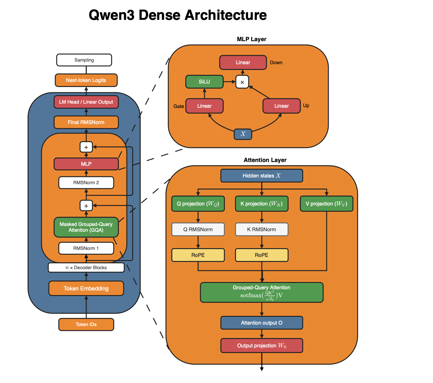
To better understand how a foundation model is deployed and parallelized across a wide range of devices, we will pick the Qwen3 model, as it is easy to understand. Its architecture is illustrated below.
We will cover how Transformer inference can combine five parallelism strategies, i.e., 5D parallelism.
Let's recall the goal of a language model, or more precisely, an autoregressive language model. Given a list of conversation messages, each with content and a role, a chat template serializes them into a prompt, and then a tokenizer maps the prompt into a vector of token IDs, or input IDs. LLM inference engines first decompose the prompt into blocks, each with its recursive hash. They then inspect the KV cache for precomputed blocks that can be reused and schedule tokens to compute during a loop. Each request has some scheduling constraints or token budget, so it may take a few steps before sampling starts, i.e., before the time to first token. Then generation starts token by token; a speculative decoder can be employed to accelerate the production of output tokens.
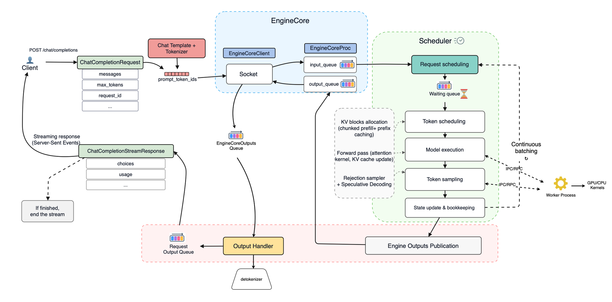
Each model is fed with an array of token IDs, which could contain tokens from different requests. For simplicity, because the goal is not to discuss continuous batching, we will assume there is only one request, as the goal is to present multidimensional parallelism. So, given input IDs, the model is provided with an input ID vector. This vector is mapped into a token embedding tensor, where each row is the embedding representation of the corresponding token. The tensor then enters the cascade of decoder layers. At the end, we have the final hidden states, which are projected into logits used to sample the next token.
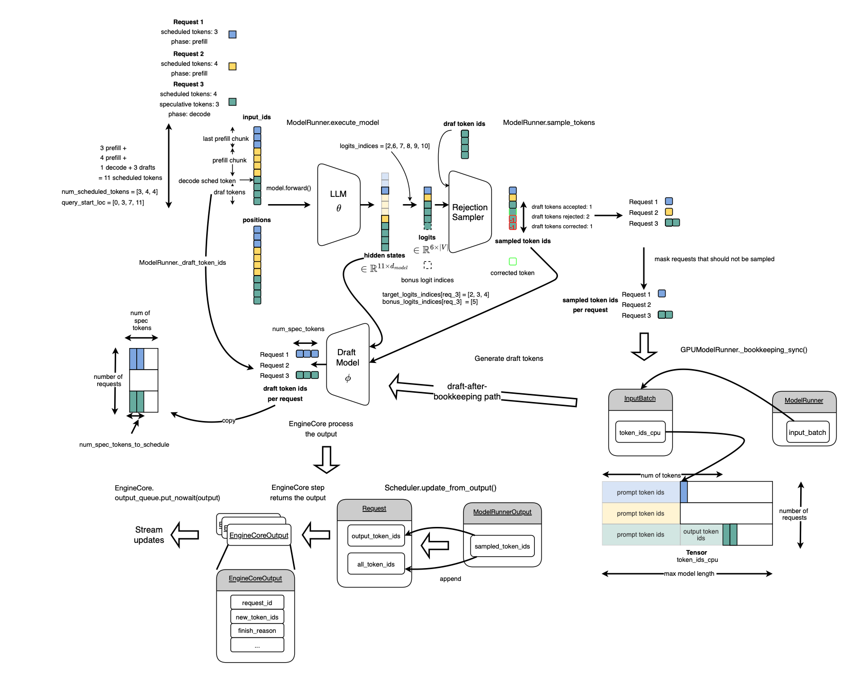
During this cascade, there are opportunities for parallelism, which will be covered one by one. But first, let's present some basics.
Tensor Parallelism (intra-layer) or TP is used in all foundation model training. In TP, we partition weight matrices across devices, along the input or output feature dimension. Let's pick a linear layer:
\[ Y = XW^T\]
For large models, \(W\) can be too large to fit inside one device, so either we need to reduce the size of the model or introduce additional GPUs that participate during the forward pass. In this case, we perform tensor partitioning, which can be row-wise or column-wise, as illustrated below.
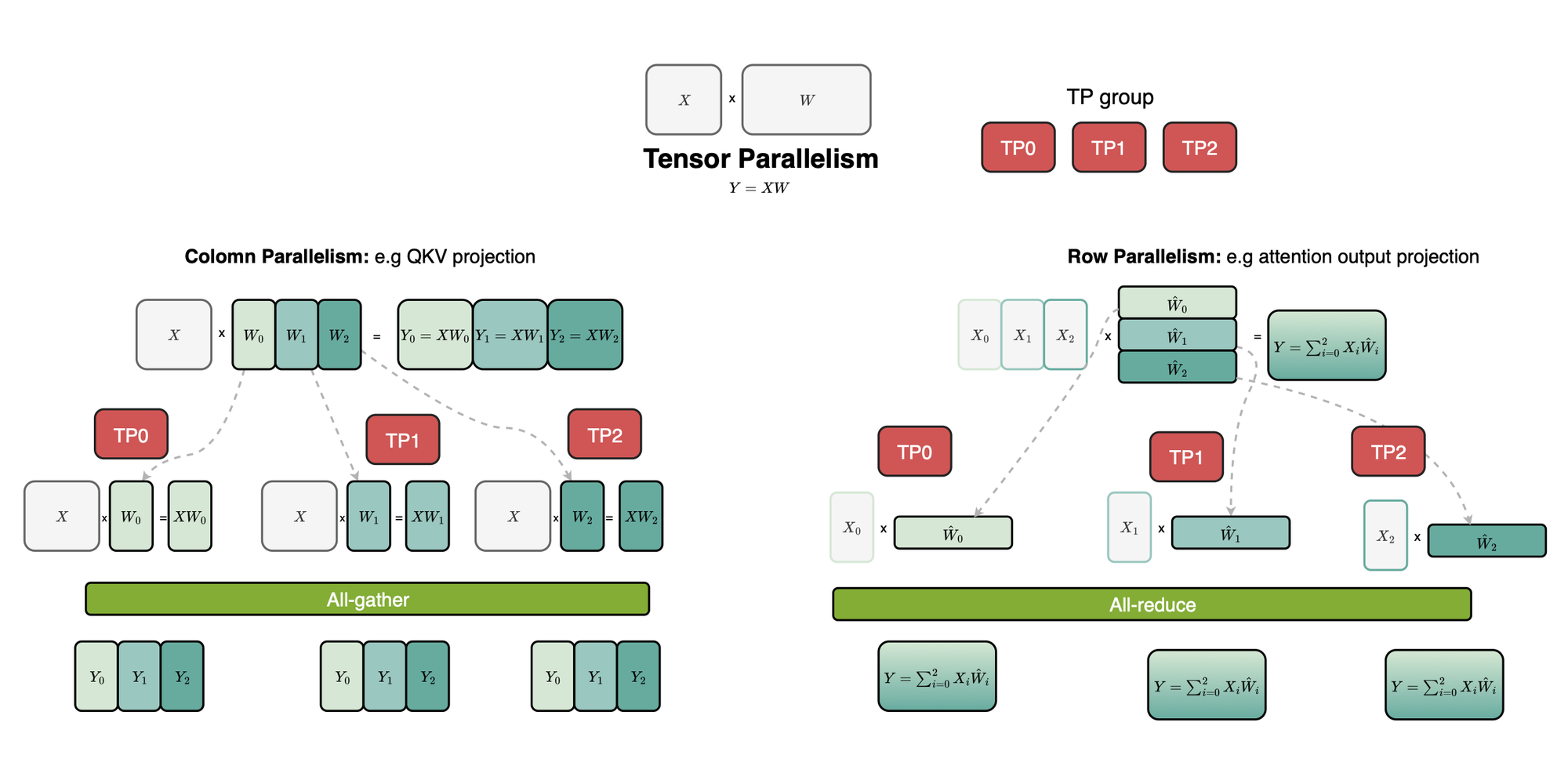
Each contributor has a TP rank, and all ranks execute their corresponding partitions of the same model. Depending on how the matrix is partitioned, each rank computes either a partition of the output or a partial contribution to the output. When communication is required, the ranks exchange or reduce their results through collective operations (all-gather or all-reduce).
Observe that while we partition \(W\), \(Y\) does not necessarily need to be replicated across TP ranks. If other compatible layers follow, we can defer communication until it is really needed and reduce communication overhead (e.g when first one uses MergedColumnParallelLinear followed by RowParallelLinear).
Tensor parallelism is used for both inference and training foundation models. We will discuss later how tensor parallelism parallelizes the multi-head attention and feed-forward blocks of Qwen3.
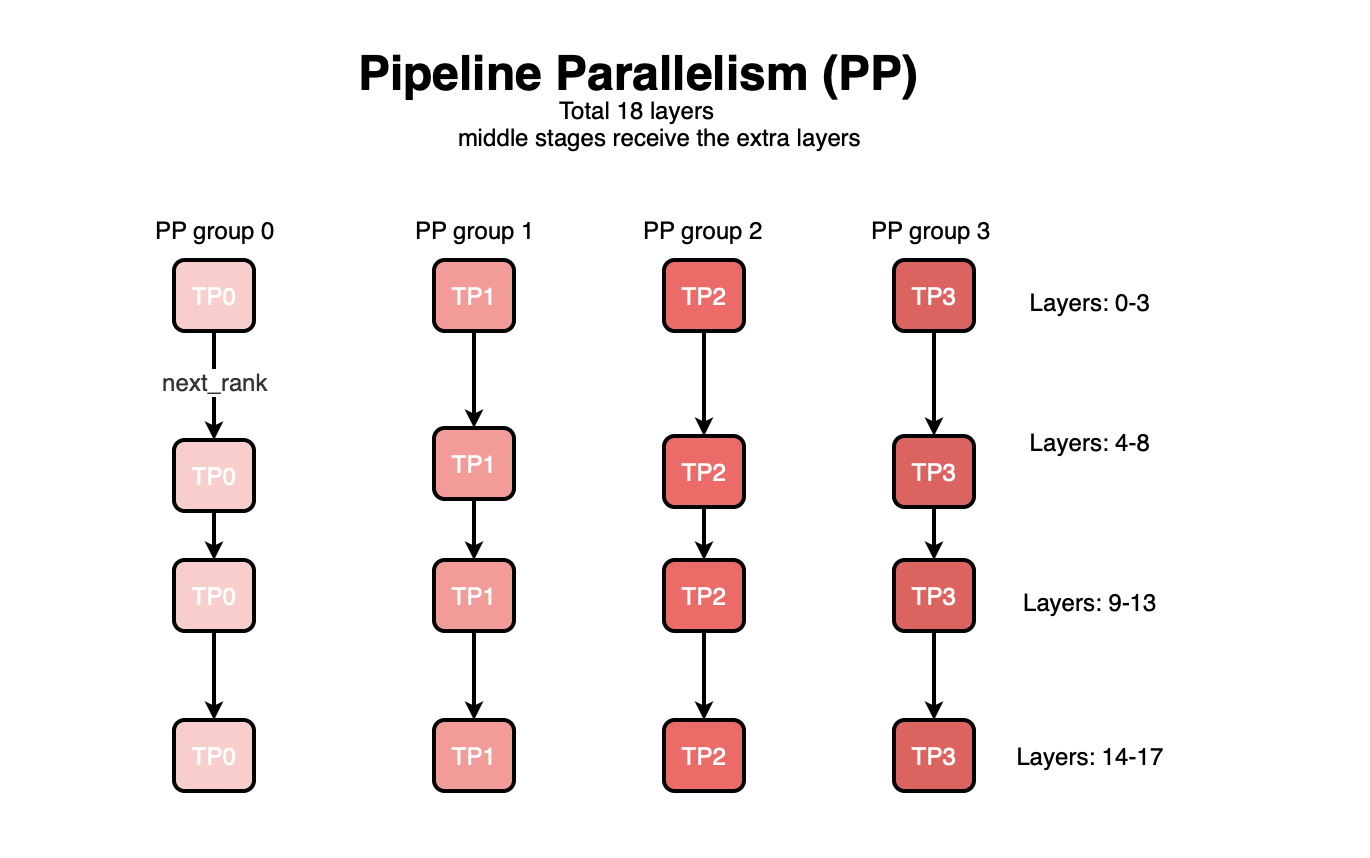
Pipeline (inter-layer) parallelism introduces another dimension where the model is seen as a series of layers, and each pipeline stage, which can contain one or multiple TP ranks, hosts and loads a subset of the model layers (the layers do not have to be partitioned equally).
PP introduces communication between consecutive pipeline stages. Each time a stage produces intermediate hidden states, they are sent to the next stage in the pipeline. This is illustrated below.
Data parallelism basically replicates the entire model across groups of GPUs. For example, without context parallelism, the total world size is:
\[ \mathrm{WorldSize} = DP \times TP \times PP\]
Each group of \(TP \times PP\) GPUs hosts one complete replica of the model, with its parameters distributed across TP ranks and PP stages. Each DP replica handles its own requests or data batches independently.
It will make more sense later, but basically, context parallelism partitions the input sequence across GPU workers along the sequence dimension.
In vLLM, prefill context parallelism (PCP) introduces additional ranks for processing different partitions of the query sequence during prefill. With PCP, the number of GPUs required for one model replica becomes:
\[ PCP \times TP \times PP\]
The entire world size then becomes:
\[\mathrm{WorldSize} = DP \times PCP \times TP \times PP\]
Some other parallelism strategies do not always add another dimension to the world size. For example, decode context parallelism (DCP), as covered later, reuses existing ranks rather than introducing an independent GPU dimension. The same applies to expert parallelism (EP).
In expert parallelism, the idea is to distribute experts across GPUs already available in the world size, i.e., across DP, PCP, and TP ranks within a pipeline stage. When the expert weights are loaded, each EP rank ignores non-local experts as will be covered later.
In vLLM, when expert parallelism uses these dimensions, the EP group size is:
\[EP = DP \times PCP \times TP\]
PP is not included in the EP group size because each pipeline stage has its own expert-parallel group.
Let \(E\) be the total number of experts in an MoE layer. With an EP degree of \(EP\), each GPU holds approximately \(\frac{E}{EP}\) experts.
EP applies only to MoE layers (e.g MLP layer in qwen3). Attention layers have no experts and still require TP, CP, or other parallelism strategies.
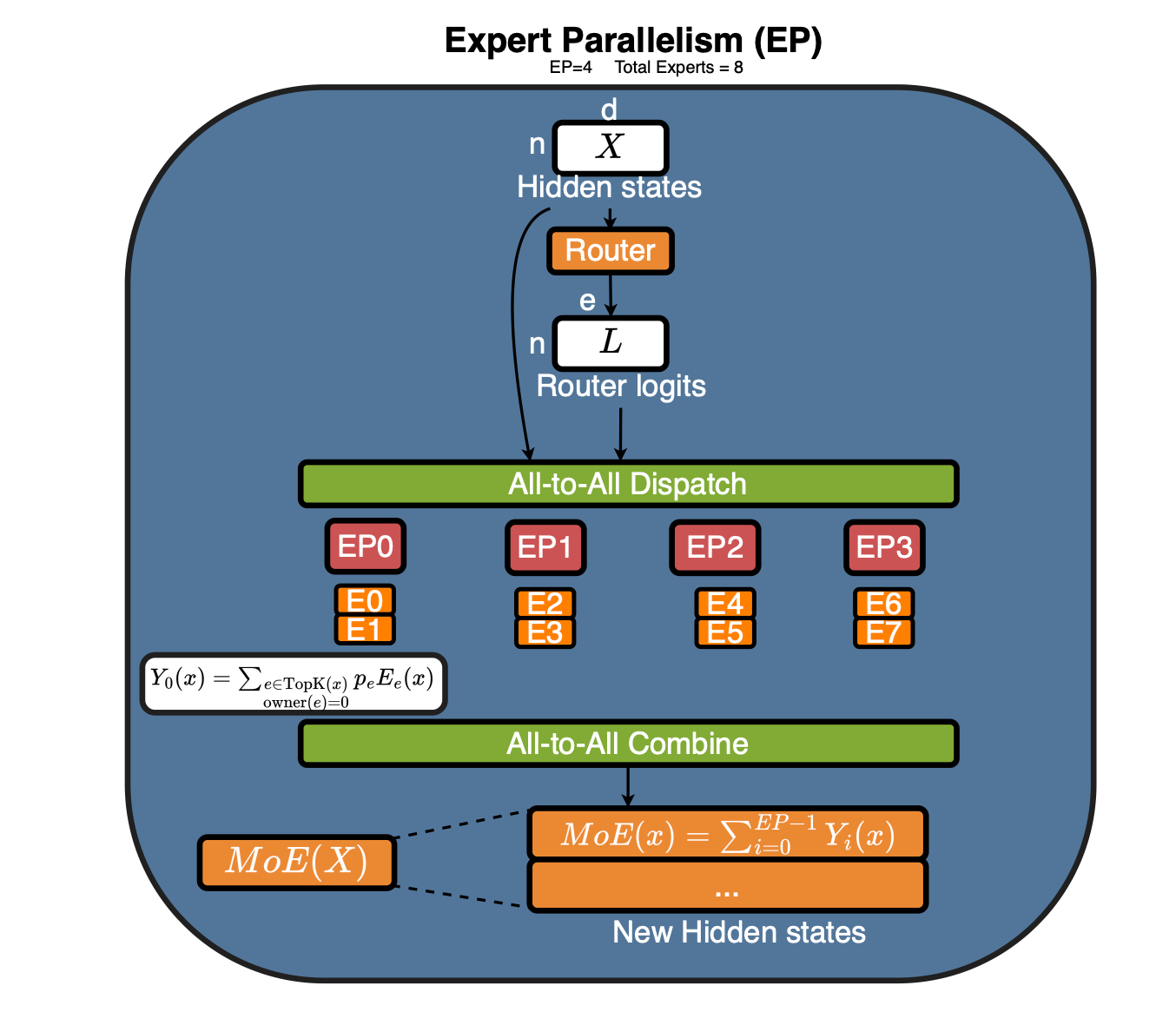
Now that we have covered how parallelism partitions layers (PP), weight matrices (TP), sequences (CP), data (DP), and experts (EP), i.e., five dimensions, let's see how we apply these strategies to Qwen3 Dense and MoE models and, at the same time, see how all of this is implemented in vLLM.
If we look at the embedding layer, it can be partitioned along the vocabulary or row dimension. Each worker then hosts a row partition of the embedding matrix. During the forward pass, invalid token IDs, i.e., token IDs that do not belong to a worker's vocabulary range, are masked and replaced with valid local indices (e.g 0) for the embedding lookup. The corresponding output embeddings are then set to zero after the lookup.
Each TP rank performs the embedding lookup and produces a tensor of shape \(n \times d\), where \(n\) is the number of input token IDs and \(d\) is the embedding dimension.
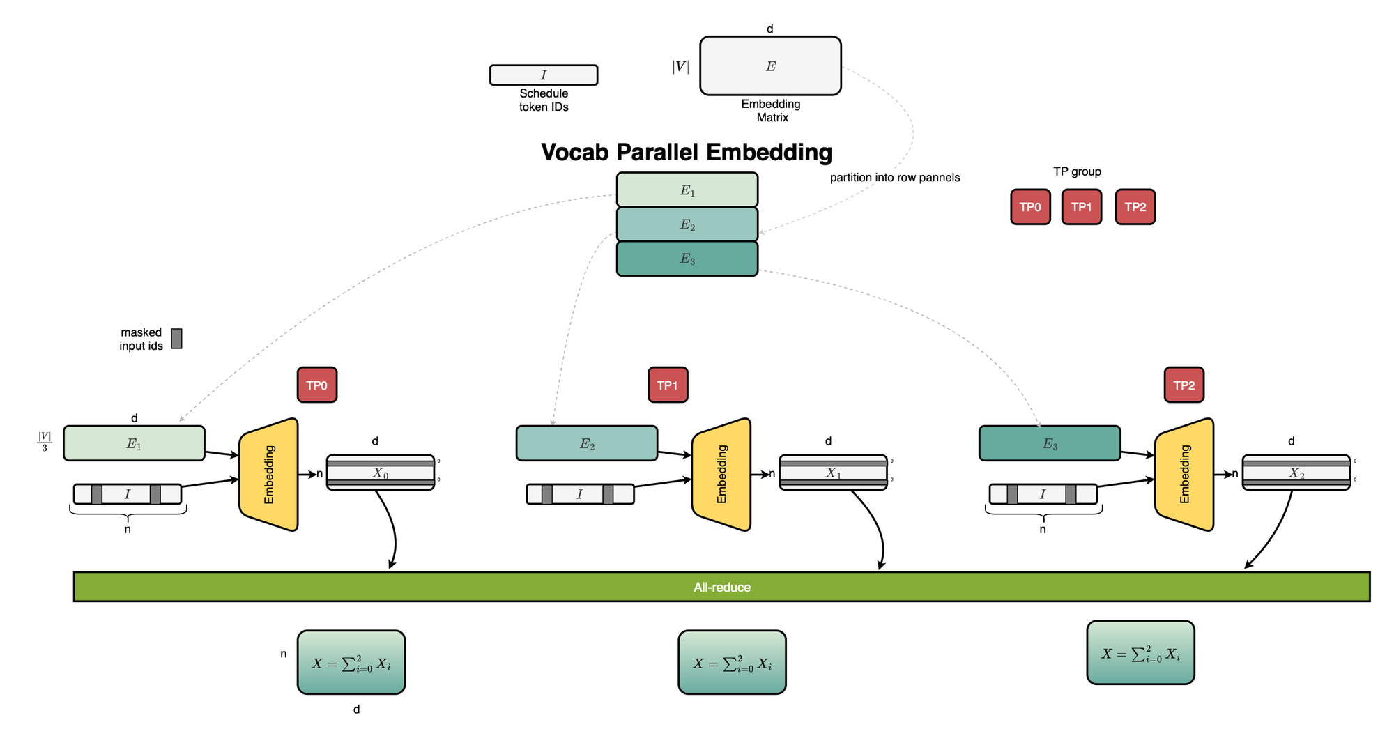
Since each token ID belongs to exactly one vocabulary partition, only one TP rank produces a nonzero embedding for that token. An all-reduce operation is then utilized to combine the outputs across all TP ranks:
\[ Y = \sum_{i=0}^{TP-1} Y_i, \qquad Y_i \in \mathbb{R}^{n \times d} \]
After the all-reduce, each TP rank has the same output embedding tensor for all scheduled input token IDs (yay).
Now, if we look at the MLP layer, it has three linear operators, the gate, up, and down projections. The gate and up projection weight matrices are partitioned by columns (the weight matrices are concatenated along the output dimension to be more precise and fused activation is used), while the down projection weight matrix is partitioned by rows.
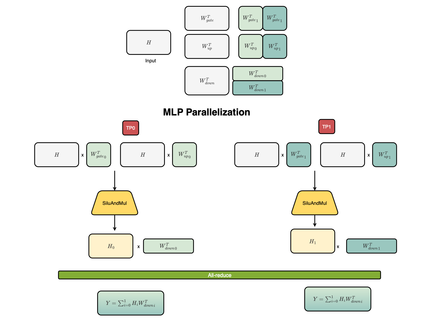
During the forward pass, each TP rank computes its local gate and up projections, applies the SiLU activation to the gate output, and then performs element-wise multiplication with the up projection output
\[ H_i = \operatorname{SiLU}(XW_{\mathrm{gate},i}^{T}) \odot (XW_{\mathrm{up},i}^{T})\]
Each TP rank then passes its local intermediate output through its partition of the down projection:
\[ Y_i = H_i W_{\mathrm{down},i}^{T}\]
An all-reduce operation is used to combine the outputs across all TP ranks:
\[ Y = \sum_{i=0}^{TP-1} Y_i \]
After the all-reduce, each TP rank has the same final MLP output tensor, which can then be used by the following operation.
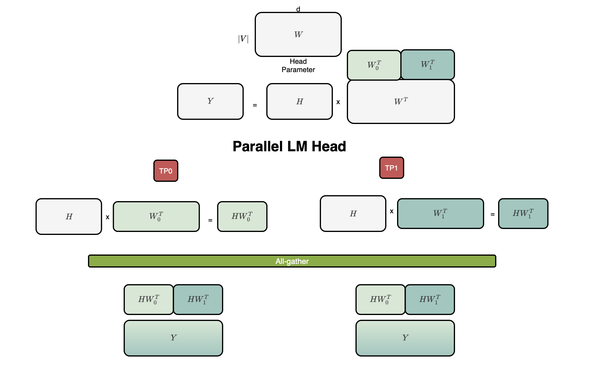
If we look at the LM head \(\texttt{ParallelLMHead}\), which also introduces a linear operator, its weight matrix is partitioned by columns across TP ranks (actually, \(\texttt{VocabParallelEmbedding}\) is reused, so row panels are employed, but due to the transpose during the linear projection, this corresponds to column panels, i.e., column parallelism). During the forward pass (or more precisely, during the computation of logits before sampling), each TP rank computes its local projection of the final hidden states into a subset of the vocabulary logits:
\[ Y_i = XW_{\mathrm{lm},i}^{T} \]
where \(X \in \mathbb{R}^{n \times d}\) represents the final hidden states and \(W_{\mathrm{lm},r}\) contains the vocabulary rows assigned to TP rank \(i\).
Each TP rank produces a tensor of shape \(n \times \frac{V}{TP}\), assuming the vocabulary size \(V\) is evenly divisible by \(TP\). An all-gather operation is then employed to concatenate the outputs along the vocabulary dimension and reconstruct the complete logits tensor (cf \(\texttt{LogitsProcessor}\) ):
\[ Y = \operatorname{AllGather}(Y_0, Y_1, \ldots, Y_{TP-1}), \qquad Y \in \mathbb{R}^{n \times V}\]
After the all-gather, each participating TP rank has the same complete logits tensor, which can then be used for sampling the next token.
For pipeline parallelism, there is no tensor partitioning of individual weight matrices across pipeline stages. Instead, each pipeline stage loads only the model layers assigned to it. Within each stage, tensor parallelism can then be applied to partition the weight matrices of those layers across the TP ranks.
class Qwen2Model(nn.Module, EagleModelMixin):
hf_to_vllm_mapper = WeightsMapper(
orig_to_new_stacked={
	# weight_name: (param_name, shard_id)
	".q_proj": (".qkv_proj", "q"),
	".k_proj": (".qkv_proj", "k"),
	".v_proj": (".qkv_proj", "v"),
	".gate_proj": (".gate_up_proj", 0),
	".up_proj": (".gate_up_proj", 1),
}
)
supports_aux_hidden_states_over_pp = True

def __init__(
self,
*,
vllm_config: VllmConfig,
prefix: str = "",
decoder_layer_type: type[nn.Module] = Qwen2DecoderLayer,
):
super().__init__()

config = vllm_config.model_config.hf_config.get_text_config()
cache_config = vllm_config.cache_config
quant_config = vllm_config.quant_config

# TODO (@robertgshaw2): see if this can be moved out
if len(set(getattr(config, "layer_types", []))) > 1:
assert config.max_window_layers == config.num_hidden_layers, (
"Sliding window for some but all layers is not supported. "
"This model uses sliding window but `max_window_layers` = {} "
"is less than `num_hidden_layers` = {}. Please open an issue "
"to discuss this feature.".format(
config.max_window_layers,
config.num_hidden_layers,
)
)

self.config = config
self.quant_config = quant_config
self.vocab_size = config.vocab_size

if (
get_pp_group().is_first_rank
or (config.tie_word_embeddings and get_pp_group().is_last_rank)
or spec_decode_needs_target_embed(vllm_config)
):
self.embed_tokens = VocabParallelEmbedding(
config.vocab_size,
config.hidden_size,
quant_config=quant_config,
prefix=f"{prefix}.embed_tokens",
)
else:
self.embed_tokens = PPMissingLayer()

self.start_layer, self.end_layer, self.layers = make_layers(
config.num_hidden_layers,
lambda prefix: decoder_layer_type(
config=config,
cache_config=cache_config,
quant_config=quant_config,
prefix=prefix,
),
prefix=f"{prefix}.layers",
)
During the forward pass, each pipeline stage executes its assigned layers and then sends the resulting intermediate hidden states to the next pipeline stage. This continues until the final stage produces the model output.
        handles = get_pp_group().isend_tensor_dict(
		output.tensors,
		all_gather_group=get_tp_group(),
		all_gather_tensors=all_gather_tensors,
)If we look at the attention layer \(\texttt{QKVParallelLinear}\), the query, key, and value projection weight matrices are partitioned by columns or the attention head dimension, while the output projection weight matrix is partitioned by rows.
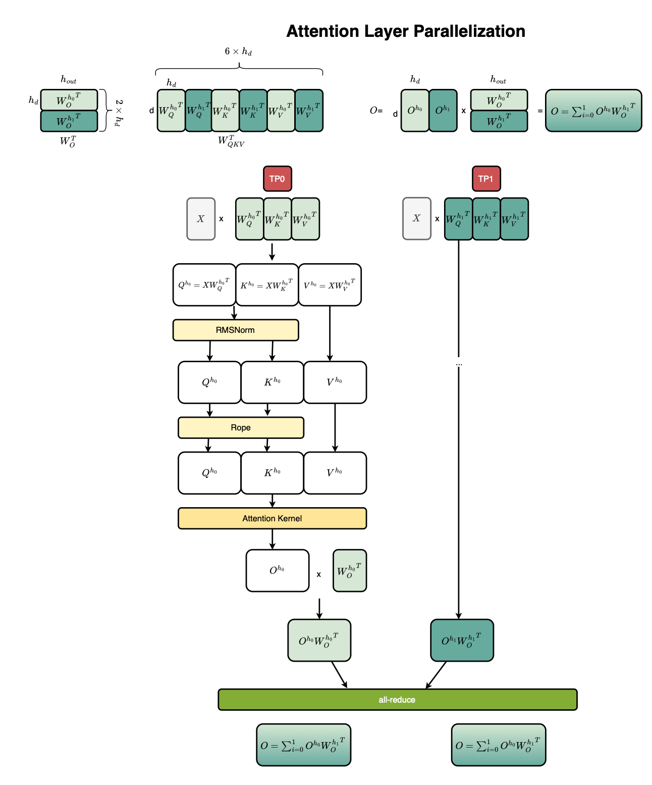
During the forward pass, each TP rank computes its local query, key, and value projections and performs attention using its assigned query heads and the corresponding key and value heads:
\[ Q_i = XW_{Q,i}^{T}, \qquad K_i = XW_{K,i}^{T}, \qquad V_i = XW_{V,i}^{T}\]
Each TP rank then computes its local attention output:
\[ H_i = \operatorname{Attention}(Q_i,K_i,V_i) \]
The local attention output is then passed through the corresponding row partition of the output projection:
\[ Y_i = H_i W_{O,i}^{T} \]
An all-reduce operation is utilized to combine the outputs across all TP ranks:
\[ Y = \sum_{i=0}^{TP-1}Y_i \]
class QKVParallelLinear(ColumnParallelLinear):
...
        self.hidden_size = hidden_size
		self.head_size = head_size
		self.v_head_size = v_head_size if v_head_size is not None else head_size
		self.total_num_heads = total_num_heads
		if total_num_kv_heads is None:
		total_num_kv_heads = total_num_heads
		self.total_num_kv_heads = total_num_kv_heads
		# Divide the weight matrix along the last dimension.
		tp_size = get_tensor_model_parallel_world_size() if not disable_tp else 1
		self.num_heads = divide(self.total_num_heads, tp_size)
		if tp_size >= self.total_num_kv_heads:
		self.num_kv_heads = 1
		self.num_kv_head_replicas = divide(tp_size, self.total_num_kv_heads)
		else:
		self.num_kv_heads = divide(self.total_num_kv_heads, tp_size)
		self.num_kv_head_replicas = 1
		input_size = self.hidden_size
		self.output_sizes = [
		self.num_heads * self.head_size * tp_size,  # q_proj
		self.num_kv_heads * self.head_size * tp_size,  # k_proj
		self.num_kv_heads * self.v_head_size * tp_size,  # v_proj
		]
		output_size = sum(self.output_sizes)
After the all-reduce, each TP rank has the same attention output tensor. For grouped-query attention (GQA), the number of key and value heads can be smaller than the number of query heads. In this case, key and value heads may be replicated across TP ranks when their number is smaller than the TP degree.
Now, if we look at decode context parallelism (DCP), the KV cache heads are still partitioned according to TP, but this time we avoid duplicating the KV cache across the participating ranks. Instead, we create DCP groups that distribute the KV cache along the sequence dimension, where each DCP rank is responsible for storing a subset of the cache positions; this means that during block allocation the DCP world size is used to determine how many blocks are needed (virtual blocks are introduced cf \(\texttt{SingleTypeKVCacheManager}\)):
	self.block_size = kv_cache_spec.block_size * self.dcp_world_size
	...
	num_required_blocks = cdiv(num_tokens, self.block_size)
If we look at the slot mapping, non-local positions will be surfaced with a magic value -1:
class ComputeSlotMappingKernel(
..
            is_local = (
virtual_block_offsets // CP_KV_CACHE_INTERLEAVE_SIZE
) % TOTAL_CP_WORLD_SIZE == TOTAL_CP_RANK
...
            slot_ids = tl.where(is_local, slot_ids, PAD_ID)
			tl.store(slot_mapping_ptr + offsets, slot_ids, mask=mask)
During cache update, the positions that are marked as non local i.e with slot mapping -1 are ignored:
template <typename scalar_t, typename cache_t, Fp8KVCacheDataType kv_dt>
__global__ void reshape_and_cache_flash_kernel(
const scalar_t* __restrict__ key,    // [num_tokens, num_heads, head_size]
const scalar_t* __restrict__ value,  // [num_tokens, num_heads, head_size]
cache_t* __restrict__ key_cache,     // NHD or HND, shape see comments below
cache_t* __restrict__ value_cache,   // same above
const int64_t* __restrict__ slot_mapping,  // [num_tokens]
const int64_t block_stride, const int64_t page_stride,
const int64_t head_stride, const int64_t key_stride,
const int64_t value_stride, const int num_heads, const int head_size,
const int block_size, const float* k_scale, const float* v_scale,
const int kv_scale_stride) {
	const int64_t token_idx = blockIdx.x;
	const int64_t slot_idx = slot_mapping[token_idx];
	if (slot_idx < 0) {
		return;
	}
This also means that attention against the KV cache is only partial, since each DCP rank has access to only its local partition of the cached keys and values. During the forward pass, an all-gather operation is first used to exchange the query heads across DCP ranks so that each rank can compute attention against its local KV cache partition.
def _forward_with_dcp(
	    query_across_dcp = get_dcp_group().all_gather(query, dim=1)
	    ...
	    context_attn_out_cor, context_lse_cor = self.dcp_combine(...
	    ...
	    merge_attn_states(...
Each DCP rank then executes the attention kernel and produces a partial attention output along with its local log-sum-exp (LSE) values. The LSEs are gathered across DCP ranks to compute the global normalization factor:
\[ L_{\mathrm{global}} = \log\left(\sum_{i=0}^{DCP-1} e^{L_i}\right) \]
Each local attention output is then corrected using the corresponding normalization factor:
\[ O_i' = O_i e^{L_i - L_{\mathrm{global}}} \]
A reduce-scatter operation is subsequently used to sum the corrected partial outputs and distribute the resulting attention heads across the participating ranks:
\[ O = \sum_{i=0}^{DCP-1} O_i' \]
Naturally, during the KV cache update, each DCP rank inserts only the keys and values corresponding to the cache positions it owns. As said ealier, vLLM uses a slot mapping to identify the physical cache locations, with invalid slot indices used to skip updates for positions that do not belong to the local rank.
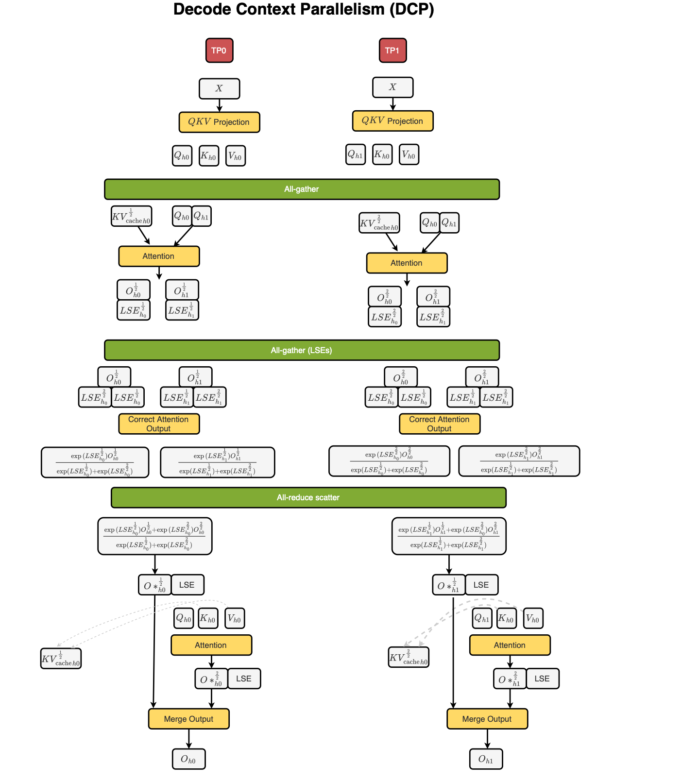
DCP reduces the KV cache memory required per rank, allowing the scheduler to allocate more KV cache blocks for requests.
This is illustrated in the figure above. During the correction of the partial attention outputs, a normalization factor is employed; details are omitted from the figure for simplicity.
In the DCP attention implementation considered here, the attention kernel is executed separately for the existing KV cache and for the newly scheduled tokens. This allows the newly computed keys and values to be processed without requiring an additional all-gather of the KV projections. The partial attention results are then combined using their corresponding LSE values to produce the final attention output.
During prefill context parallelism (PCP), each PCP rank processes a partition of the input token sequence.
class PCPManager:
	...
	  def partition_batch(
        local_gather_idx = self._padded_gather_idx[
		rank_token_start : rank_token_start + num_local_tokens_padded
		]
		self._local_gather_idx = local_gather_idx
		torch.index_select(
		global_batch.input_ids,
		0,
		local_gather_idx,
		out=input_buffers.input_ids[:num_local_tokens_padded],
		)
With TP in place, each TP rank is also assigned a subset of the attention heads.
During the forward pass, each PCP rank computes the query, key, and value projections for its local tokens. However, since we are dealing with causal attention in an autoregressive language model, each query token must be able to attend to all preceding tokens, including those processed by other PCP ranks.
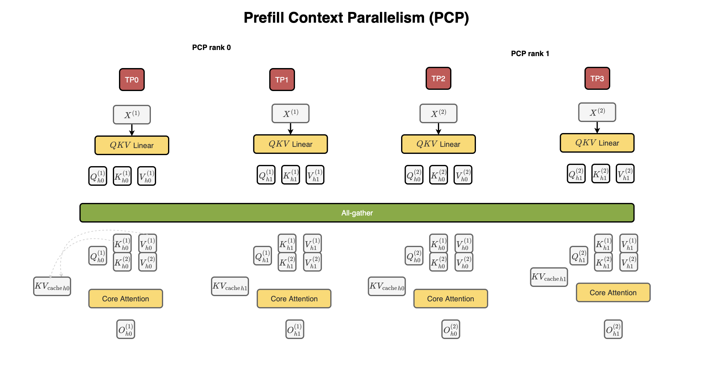
To achieve this, an all-gather operation is used across the PCP ranks to exchange the newly computed keys and values. The gathered keys and values are then used to update the KV cache, ensuring that the attention kernel has access to the required context.
def _gather_prefill_cache_inputs(
	...
	gathered_prefills = tuple(
	pcp_group.all_gather(tensor[num_decode_tokens:].contiguous(), dim=0)
	for tensor in tensors
	)
	...
The attention kernel is then executed as usual, with each PCP rank computing attention for its assigned query tokens while respecting the causal mask.
PCP can also be combined with DCP. However, not all possible configurations are supported by vLLM. In the implementation considered here, the supported configurations are restricted to cases where the DCP degree is equal to the PCP degree or to the product of the PCP and TP degrees:
\[ DCP = PCP \] or \[ DCP = PCP \times TP\]
In both cases, DCP reuses existing parallel ranks rather than introducing additional GPUs into the world size.
def _prefill_query_all_gather(self, attn_metadata, prefill_query):
		if self.use_pcp:
		prefill = attn_metadata.prefill
		assert prefill is not None
		chunked_context = prefill.chunked_context
		assert chunked_context is not None and chunked_context.pcp_query_restore_idx is not None
		# PCP splits the query sequence, not the history KV cache. Restore
		# all current queries before computing each DCP history shard.
		prefill_query = self.pcp_group.all_gather(prefill_query.contiguous(), dim=0)
		prefill_query = torch.index_select(prefill_query, 0, chunked_context.pcp_query_restore_idx)
		(prefill_query,) = self._dcp_all_gather_fragments(prefill_query, dim=1)
return prefill_queryGiven EP ranks participating as workers, each rank holds the local experts assigned to it, in the simplest case using a linear placement strategy
	# Create an expert map for the local experts
	if expert_placement_strategy == "linear":
	start_idx = ep_rank * base_experts + min(ep_rank, remainder)
	expert_map[start_idx : start_idx + local_num_experts] = torch.arange(
	0, local_num_experts, dtype=torch.int32
	)
If an expert is not local, its weights are skipped during loading
	if expert_id == -1 and not use_global_sf:
	# Failed to load this param since it's not local to this rank
	return False if return_success else None
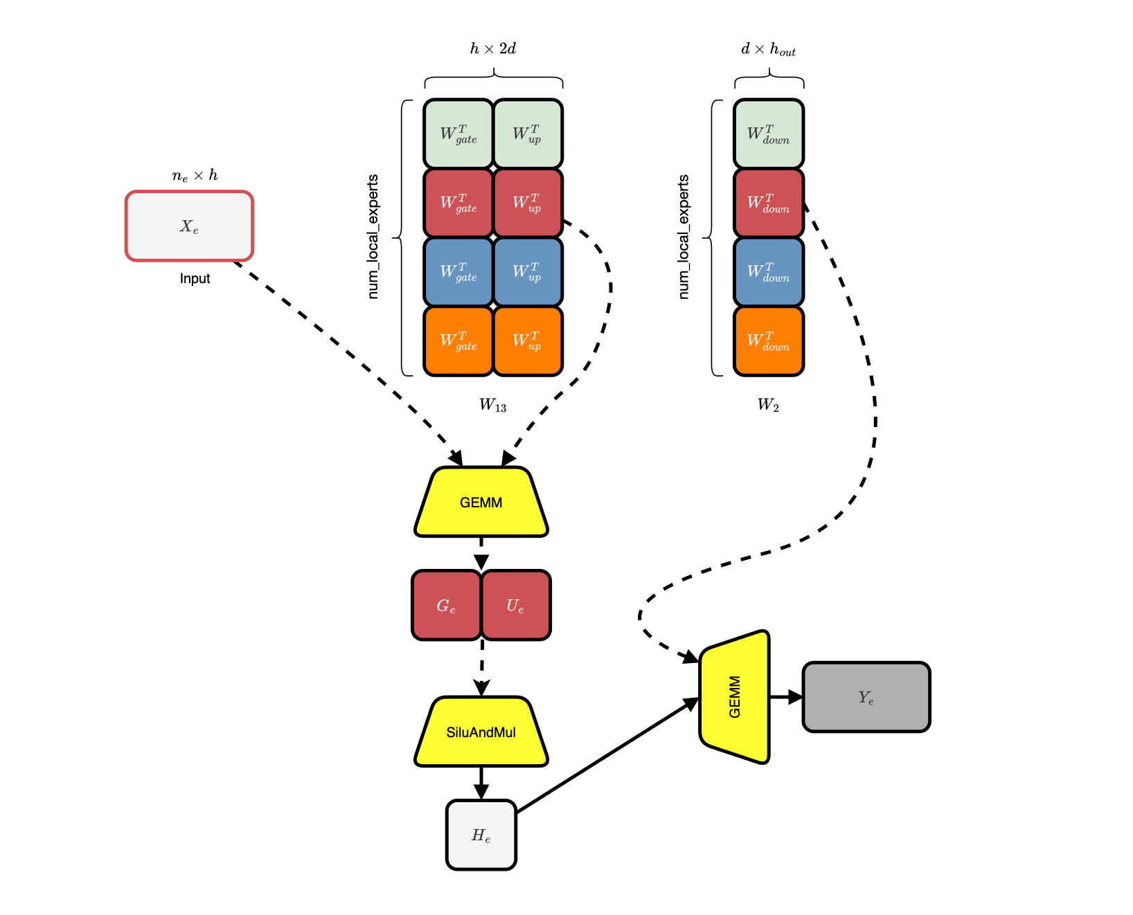
Each expert in Qwen basically consists of three weight matrices: W1 (gate), W3 (up), and W2 (down). W1 and W3 are packed together into W13
w13_weight = torch.nn.Parameter(
	torch.empty(
	num_experts,
	w13_up_dim,
	hidden_size,
	dtype=params_dtype,
	),
	requires_grad=False,
	)

	...

	w2_weight = torch.nn.Parameter(
	torch.empty(
	num_experts,
	hidden_size,
	intermediate_size_per_partition,
	dtype=params_dtype,
	),
	requires_grad=False,
	)
Then, during the forward pass, given a tensor where each row represents a token, routing logits are produced using a gate layer, and a Top-K operator is applied to select the experts (a dispatch primitive is used to send token hidden states and routing information to the corresponding EP ranks when needed; in the naive scenario, the required data is gathered across all participating workers).
def _maybe_dispatch(
self,
hidden_states: torch.Tensor,
router_logits: torch.Tensor,
) -> tuple[torch.Tensor, torch.Tensor]:
	# For naive dispatch/combine Dp/Ep, dispatch the hidden states and
	# router logits to all experts.
	# NOTE: this will be removed once all kernels are migrated into the
	# MoEKernel framework.
	if self.do_naive_dispatch_combine:
		result = get_ep_group().dispatch_router_logits(
		hidden_states,
		router_logits,
		self.moe_config.is_sequence_parallel,
		)
		assert len(result) == 2
		hidden_states, router_logits = result

	if (
	self.moe_config.pcp_size > 1
	and not self.moe_config.moe_parallel_config.use_all2all_kernels
	):
		hidden_states = get_pcp_group().all_gather(hidden_states, dim=0)
		router_logits = get_pcp_group().all_gather(router_logits, dim=0)

	return hidden_states, router_logits
Then, each EP rank batches token assignments by expert, and two fused MoE kernel invocations are employed to perform the projections, with an activation kernel in between. The first kernel computes the gate and up projections, while the second computes the down projection. Finally, the expert outputs are accumulated according to their original token assignments, restoring the token order. This approach uses GEMM instead of GEMV, with better efficiency when enough tokens are available per expert. A combine operation is then used to aggregate the results across EP ranks when necessary (you can inspect \(\texttt{class TritonExperts}\) and \(\texttt{fused\_moe\_kernel}\) for more details).
That's it.
If you find a mistake, do not hesitate to reach out. I will anyway publish my new notes (including vLLM internals E2E) soon at https://books.deep-kondah.com as I cover more subjects with corrections if spotted.