The goal of this post is to briefly present how multi-agent systems emerged by looking at some of the history and the cognitive backbone of AI or LLM-powered agents. An autoregressive language model, which will be denoted as \(p_\theta\) (or \(\pi_\theta\) in RL terminology), is a

The goal of this post is to briefly present how multi-agent systems emerged by looking at some of the history and the cognitive backbone of AI or LLM-powered agents.
An autoregressive language model, which will be denoted as \(p_\theta\) (or \(\pi_\theta\) in RL terminology), is a model trained on massive corpora to comprehend the distribution that governs the world's language space by learning how to predict the next word or token, \( p_\theta(x_t \mid x_{<t})\).
The conditional distribution \(p_\theta(x_t \mid x_{<t})\) is modeled by a deep neural network, where the representation of the last token is used to produce the logits parameterizing the categorical distribution over the vocabulary (the set of possible output tokens forms the vocabulary). By learning each conditional distribution, the model effectively learns the joint distribution over sequences through the chain rule:
\[
p_\theta(x)
=
\prod_{t=1}^{T}
p_\theta(x_t \mid x_{<t}),
\]
where \( x=(x_1,x_2,\ldots,x_T) \).
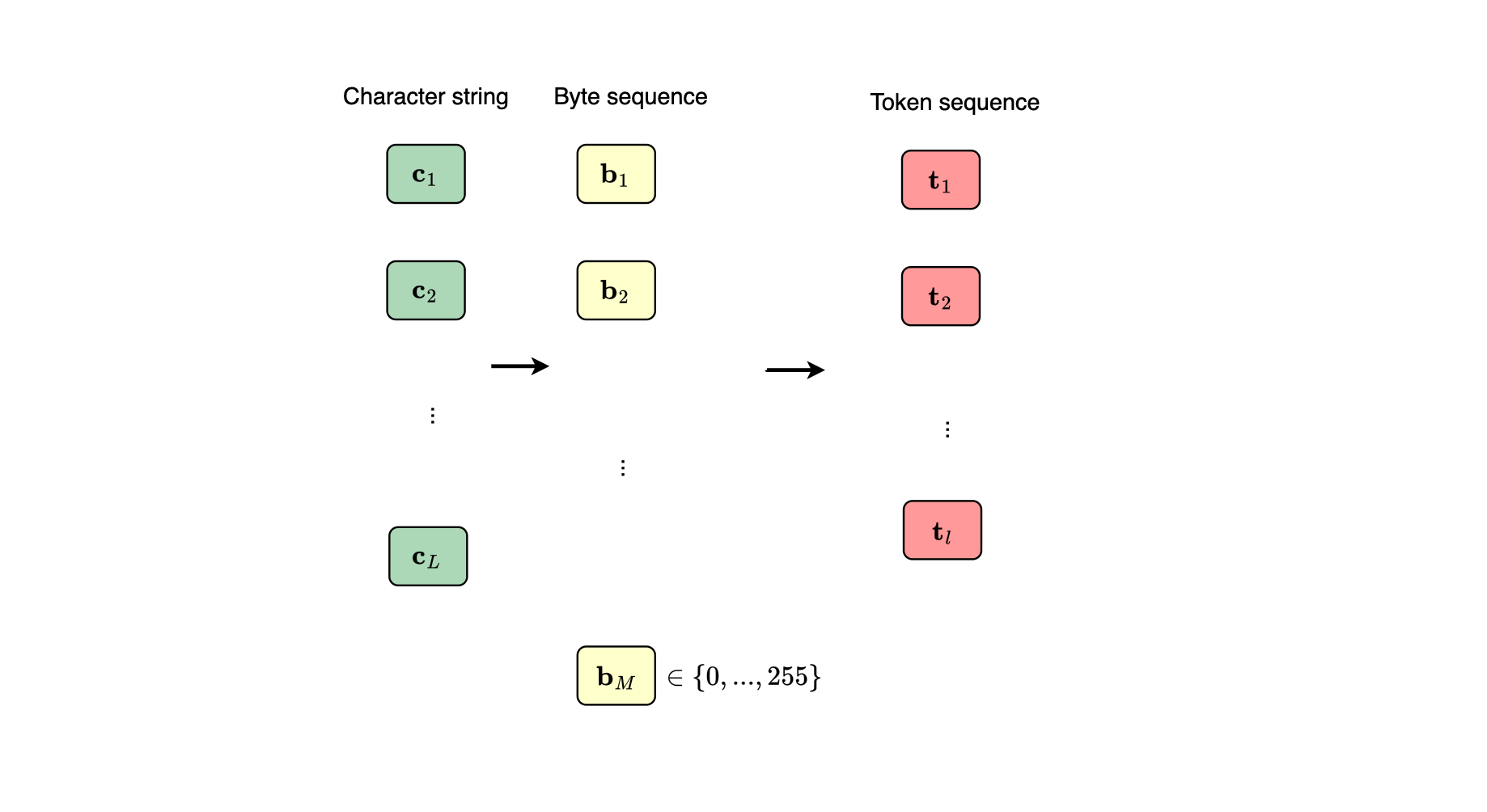
Basically, you want a model that, once conditioned on say "I spent my summer in Morocco, it is very," predicts that the next word (or set of tokens) is "hot" and not "cold".
Previous generations of language models like Recurrent Neural Networks or RNNs, were used to train language models, but in addition to their sequential nature, which limits parallelization during training and inference, training could be slow and vanishing gradients were a significant problem; information from distant words or tokens in the context could be lost, and later representations were only weakly influenced by earlier tokens, leading to the long-range dependency problem.
Formally, the gradient of the loss with respect to an earlier hidden state \(h_k\) is
\[
\frac{\partial \mathcal{L}}{\partial h_k}
=
\frac{\partial \mathcal{L}}{\partial h_N}
\frac{\partial h_N}{\partial h_{N-1}}
\frac{\partial h_{N-1}}{\partial h_{N-2}}
\cdots
\frac{\partial h_{k+1}}{\partial h_k}
\]
Because this gradient is obtained through a product of many Jacobians, its magnitude can become very small as it is propagated through a long sequence. Since a gradient or Jacobian measures a rate of change, a very small \(\frac{\partial \mathcal{L}}{\partial h_k}\) means that a change in an earlier token representation \(h_k\) has very little effect on the loss, making it hard for the model to learn long-range dependencies.
Later, the Attention mechanism was introduced. Basically, instead of heavily compressing the history and hoping the model would manage to preserve what is needed, each token has the ability to inspect and look at previous tokens, that is, the model is equipped to focus on different parts of a sequence. More specifically, the model learns an attention distribution for each token with respect to other tokens in the context to form a more powerful contextualized embedding that is used as a representation for future word or token prediction.
The benefits of the introduction of transformer architecture includes training speed up and encoding of long-range dependencies.
Transformer blocks make use of attention, including self-attention and cross-attention, while decoder-only Transformers use self-attention and are, for instance, the backbone of GPT-like models.
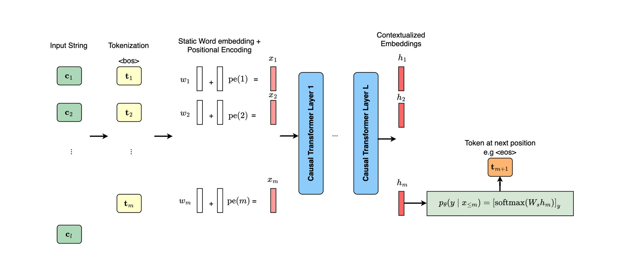
If we look at what a Transformer decoder does, it basically learns via maximum likelihood and backpropagation. Given a sequence mapped to a set of tokens,
each conditional distribution \(p_\theta(x_t \mid x_{<t})\) is modeled by the same shared deep neural network, where the contextualized representation at position \(t-1\) is projected into logits and a softmax produces a categorical distribution over the vocabulary. The unsupervised language-modeling loss is then given by the negative log-likelihood:
\[
\mathcal{L}_{\mathrm{LM}}(\theta)
=
-\mathbb{E}_{x\sim\mathcal{D}}
\left[
\sum_{t=1}^{T}
\log p_\theta(x_t \mid x_{<t})
\right].
\]
For a mini-batch \(\mathcal{B}\), this can be written as
\[
\mathcal{L}_{\mathrm{LM}}(\theta)
=
-\frac{1}{|\mathcal{B}|}
\sum_{x\in\mathcal{B}}
\sum_{t=1}^{T}
\log p_\theta(x_t \mid x_{<t})
\]
Minimizing this loss through backpropagation is equivalent to maximizing the likelihood of the training sequences under \(p_\theta\).
So, we can say that language models based on Transformers learn the conditional distributions, or probability mass over tokens, and thus, by the chain rule, learn the likelihood of sequences.
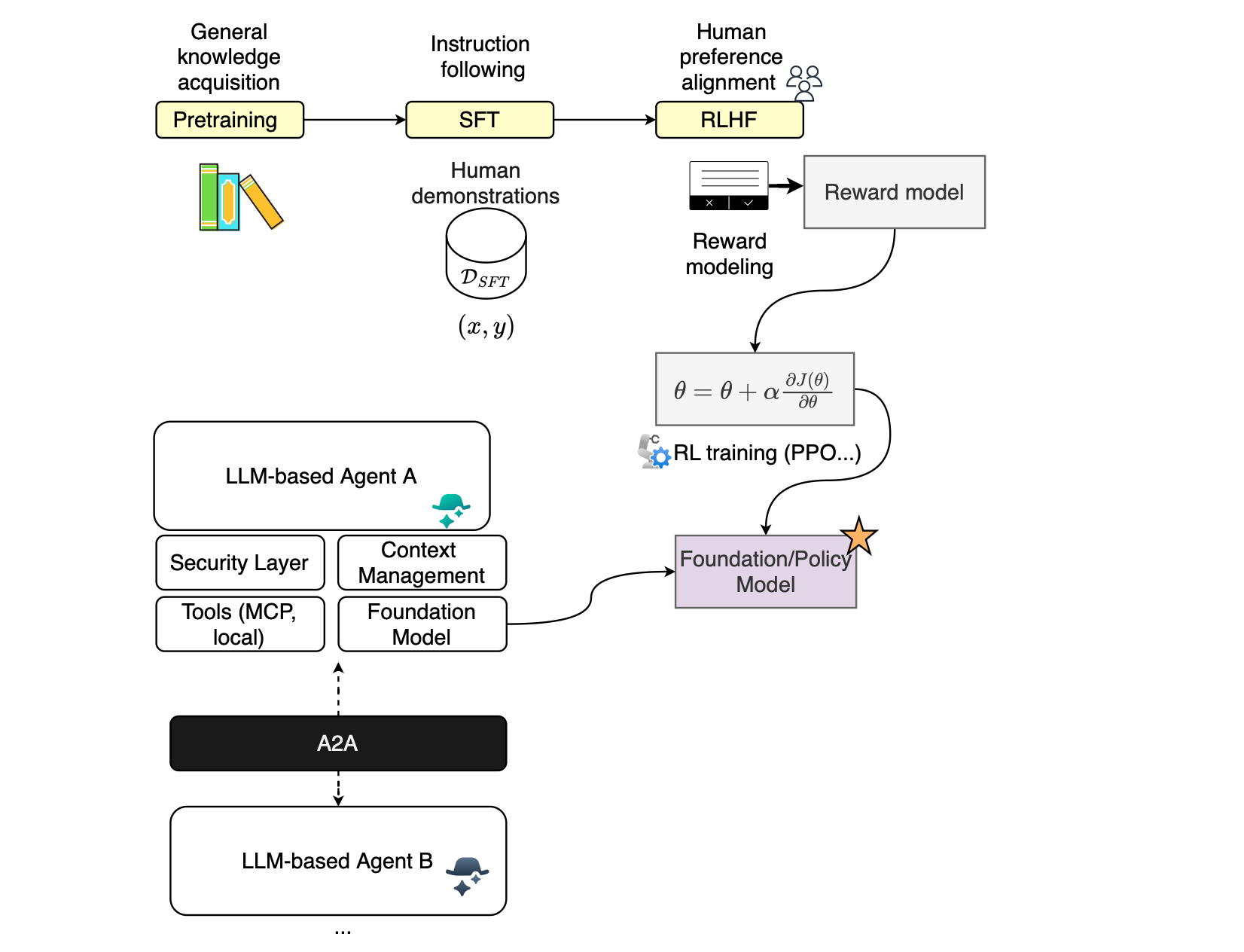
LLMs, build on the Transformer architecture, are trained on vast amounts of text corpora, and they are made very large, hence the term "large language models'' (cf. scaling laws). They typically undergo pretraining first, where the model learns syntax, semantics, common patterns, and a broad range of knowledge. Pretraining is typically followed by Supervised Fine-Tuning (SFT), where the model is trained on prompt-response pairs \((x,y)\) to learn how to follow instructions. The SFT objective is
\[
\mathcal{L}_{\mathrm{SFT}}(\theta)
=
\mathbb{E}_{(x,y)\sim\mathcal{D}_{\mathrm{SFT}}}
\left[
-\sum_{t=1}^{T}
\log p_\theta
\left(
y_t\mid x,y_{<t}
\right)
\right]
\]
Next, LLMs are typically taught to better align with human values using Reinforcement Learning (RL).
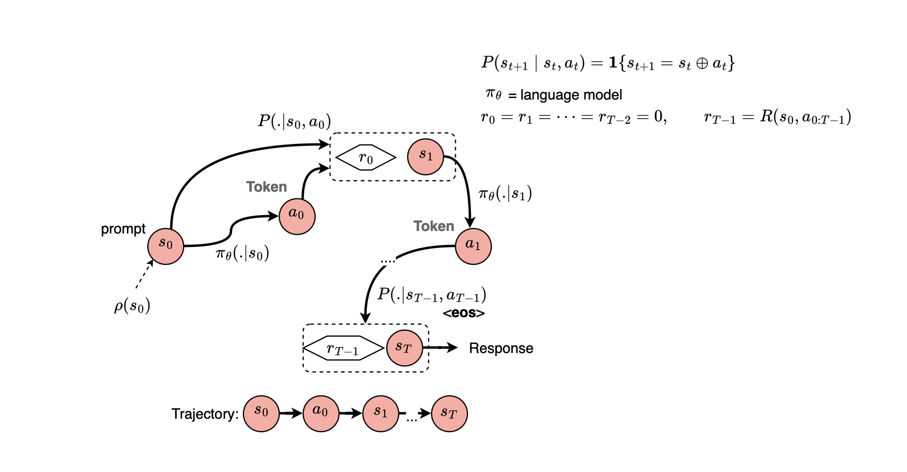
This can involve first training a reward model \(R_\psi\) from human preference data. Given a preferred response \(y_w\) and a less-preferred response \(y_l\), the reward-model objective is
\[
\mathcal{L}_{\mathrm{RM}}(\psi)
=
-\mathbb{E}_{(x,y_w,y_l)\sim\mathcal{D}_{\mathrm{RM}}}
\left[
\log
\sigma
\left(
R_\psi(x,y_w)-R_\psi(x,y_l)
\right)
\right]
\]
The language model is then cast as a policy \(\pi_\theta\), where, for a generated response
\[
y=(y_1,\ldots,y_T),
\]
the state and action at time \(t\) are
\[
s_t=(x,y_{<t}),
\qquad
a_t=y_t,
\]
and therefore
\[
\pi_\theta(a_t\mid s_t)
=
\pi_\theta(y_t\mid x,y_{<t}).
\]
An initial KL-regularized RL objective can be written as
\[
\max_{\theta}
\;
\mathbb{E}_{x}
\mathbb{E}_{y\sim\pi_\theta(\cdot\mid x)}
\left[
R_\psi(x,y)
-
\beta
D_{\mathrm{KL}}
\left(
\pi_\theta(\cdot\mid x)
\;\Vert\;
\pi_{\mathrm{ref}}(\cdot\mid x)
\right)
\right]
\]
where \(\pi_{\mathrm{ref}}\) is typically the reference policy obtained after SFT. PPO can then be used to optimize the policy while constraining excessively large policy updates.
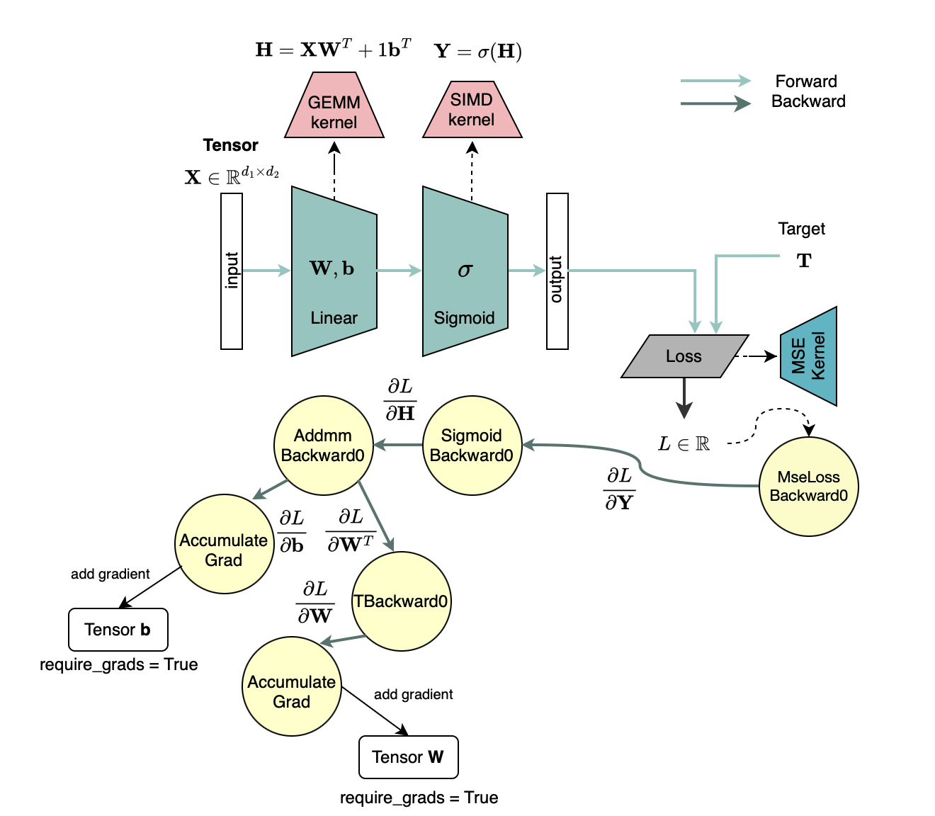
With PyTorch, training LLMs is relatively easy thanks to automatic differentiation, where the backward computation graph is created on the fly and executed when invoking backward() on the loss tensor.
Once an LLM is equipped to follow instructions, it can be trained to use tool calls, and this is what made function calling more reliable and structured, although tool use was already possible through in-context learning.
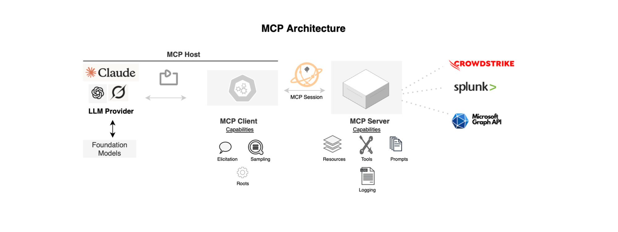
MCP or Model Context Protocol was later introduced to avoid fragmented integrations, where each application exposes APIs to the LLM differently, and to make it easier to connect external tools without modifying every application-specific integration (sometimes you can't even modify it e.g Claude code). Of course, this also opens the door to injection attacks.
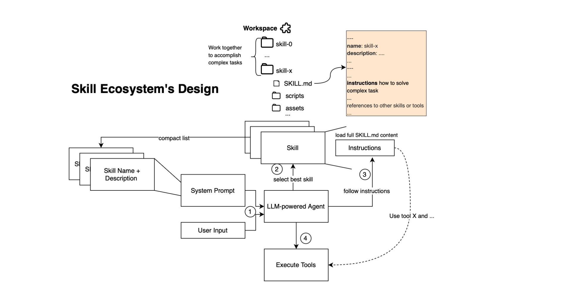
Later, Skills were introduced as as a way to augment agents with procedural knowledge without fine-tuning model parameters. Instead of updating weights, one can guide agent behavior at inference time using modular, reusable artifacts known as skills or agent skills. These bundles encode task-specific workflows, instructions, and auxiliary resources like references or assets dynamically loaded when deemed relevant by the underlying agent.
Additionally, LLMs can also be fine-tuned to reason. This is why they serve as the primary reasoning engine for agents. Large Reasoning Models are basically LLMs trained to produce a Chain-of-Thought or CoT sub trajectory, often delimited by special tokens, before producing the final answer to a prompt (the internal reasoning is typically hidden form users).
LLMs are also commonly optimized using MoE or Mixture of Experts, which consists of conditional computation. Basically, only a portion of the model, typically a subset of FFN experts, participates in the computation for a given token, which can improve computational efficiency during training and inference.
Distillation is another technique used to transfer knowledge from a teacher model to a student model by adding a loss term that encourages the student to mimic the probability distribution of the teacher, thereby learning information about other classes or tokens captured by the teacher rather than only the hard target.
While LLM inference is forced to obey the autoregressive property by generating one token at a time, during training, teacher forcing is used; the entire known sequence can be processed in parallel while a causal mask forces each token representation to attend only to preceding tokens and switch off attention to future tokens.
Using column convention, the attention operation is
\[
\operatorname{Attention}(X)
=
V
\left[
\operatorname{softmax}
\left(
\frac{Q^\top K}{\sqrt{d_k}} + M
\right)
\right]^\top
\]
where the causal mask \(M\) is defined as
\[
M_{ij}
=
\begin{cases}
0, & j \leq i,\ \
-\infty, & j > i.
\end{cases}
\]
Thus, although the representations of all tokens can be computed in parallel during training, token \(i\) can only attend to itself and preceding tokens. This is a key difference from sequential models such as RNNs.
Retrieval-Augmented Generation (RAG) is used to ground LLM responses in retrieved external information. This can be represented as
\[
p_\theta
\left(
y \mid p, \operatorname{retrieve}(q)
\right),
\]
where \(p\) is the prompt and \(\operatorname{retrieve}(q)\) represents the tokens corresponding to the documents or contextual information retrieved for a query \(q\). The generated output is therefore conditioned on both the prompt and the retrieved context, which can reduce hallucinations and improve factual grounding.
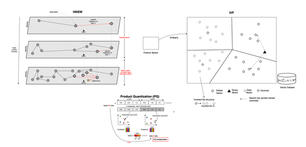
For example, vector-based RAG uses contextualized embeddings produced by Transformer-based models to represent document chunks and indexes these embeddings in an Approximate Nearest Neighbor (ANN) index, enabling efficient retrieval at query time.
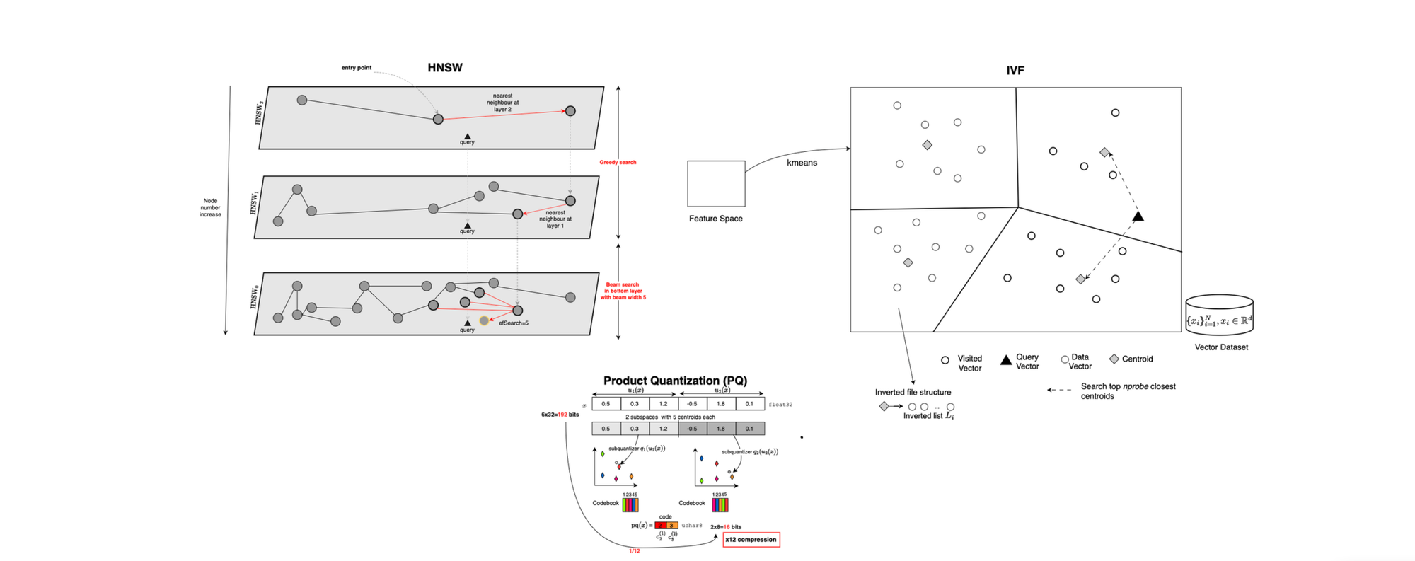
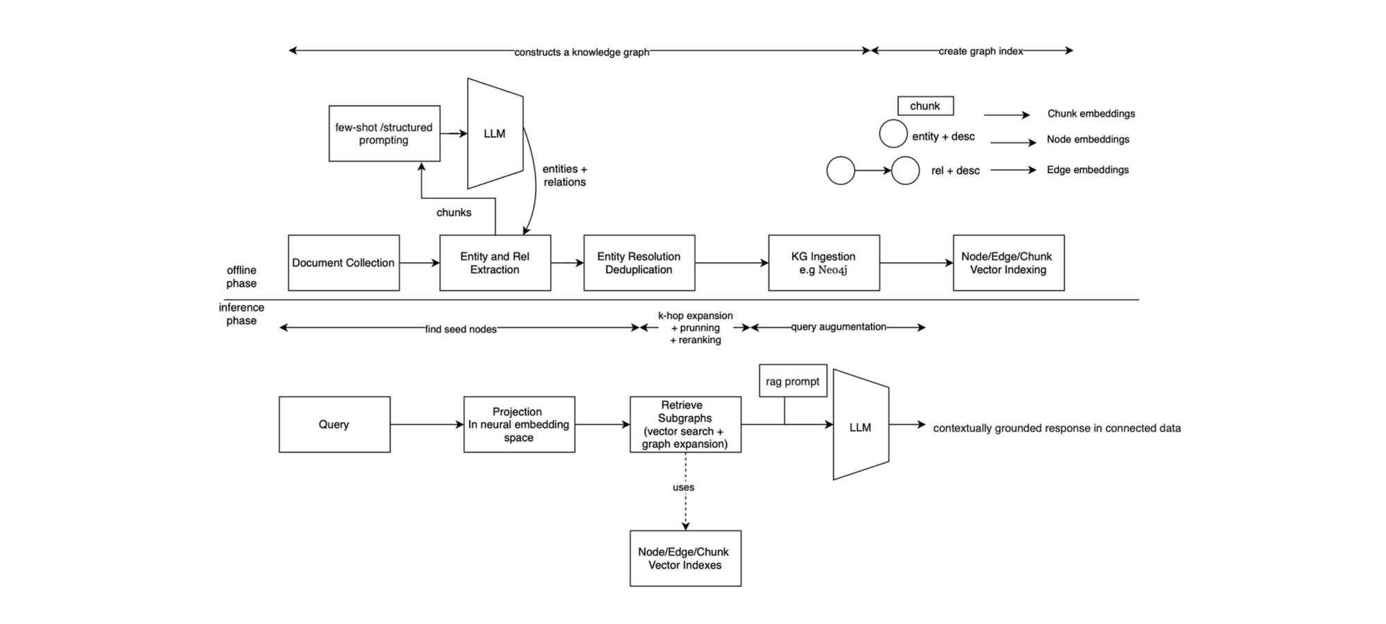
Traditional RAG has several drawbacks, including hallucinations caused by the context being polluted with irrelevant information retrieved from the ANN index, which can be mitigated through re-ranking. Moreover, retrieved chunks are typically treated in isolation. This is where Graph-Based Retrieval-Augmented Generation or GraphRAG comes into play. The basic idea is to use a knowledge graph as a basis for retrieval, for example, by selecting relevant anchor nodes and expanding their neighborhoods to construct the context used for generation. GraphRAG can itself incorporate vector-based retrieval by embedding graph nodes, meaning that semantic search through vector databases can still be used. However, the knowledge graph additionally captures intricate relational information between entities, allowing more complex queries to be addressed and enabling multi-hop reasoning, as multi-hop relationships can be explicitly uncovered by traversing the knowledge graph.
Once an LLM knows how to distinguish between a system input message, which contains instructions and a persona, and other types of messages such as user messages and tool responses, the LLM can be called recursively in a loop (called stacking), with the conversation history containing the trajectory generated so far, and thus an agent is born. An agent is simply a foundation model, a tool set, an execution environment, and a loop called the agent loop.
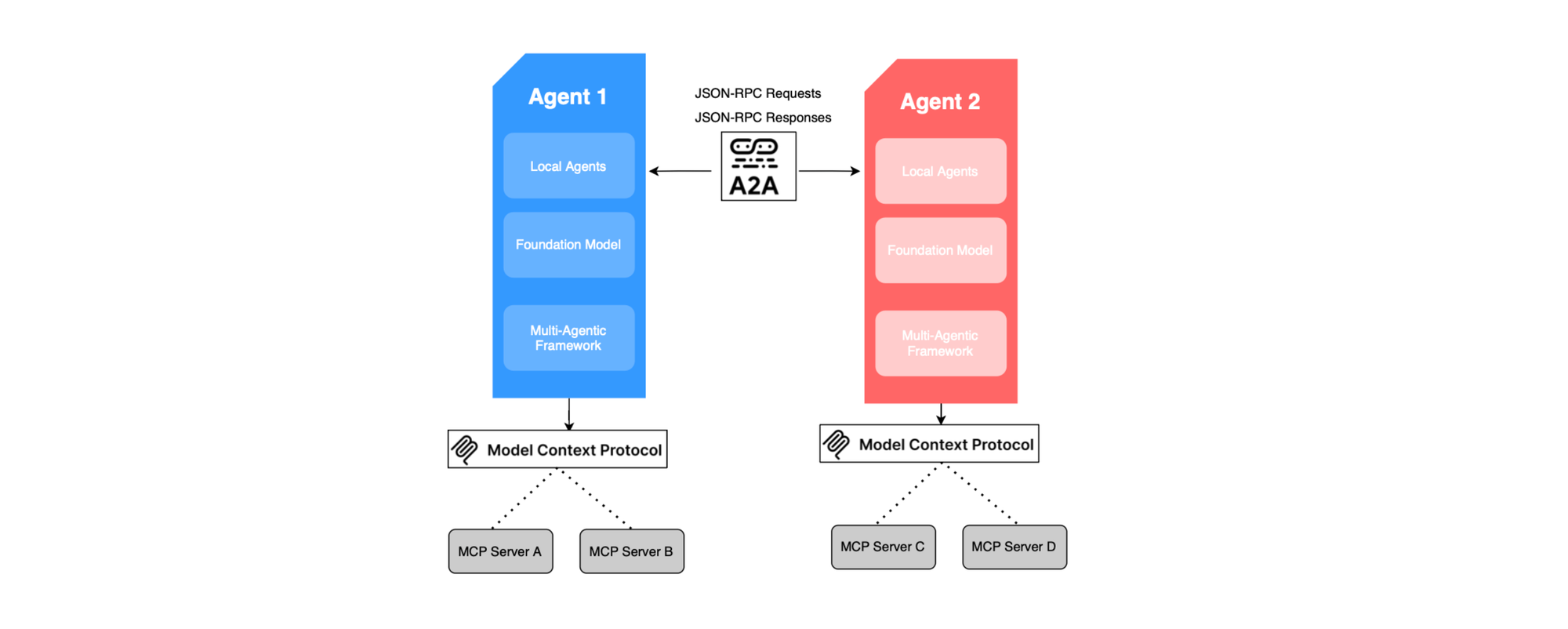
Once you have an agent, you can introduce multiple agents and connect them, for example locally through tools using patterns such as agent-as-a-tool or handoffs. You can then define a pattern for your multi-agent system and break down a complex problem so that it can be solved by multiple specialized agents, each potentially having its own tool set, history, and foundation model.
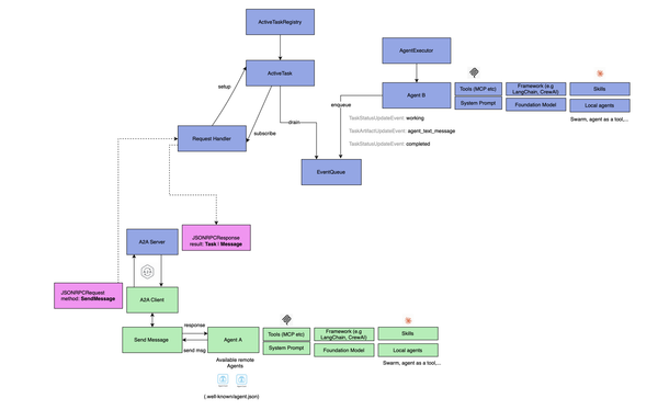
A2A agents are basically agents that expose an A2A interface, a standardized interface through which agents can exchange messages. This is similar to exposing an external tool, except that what is being exposed is an external agent.
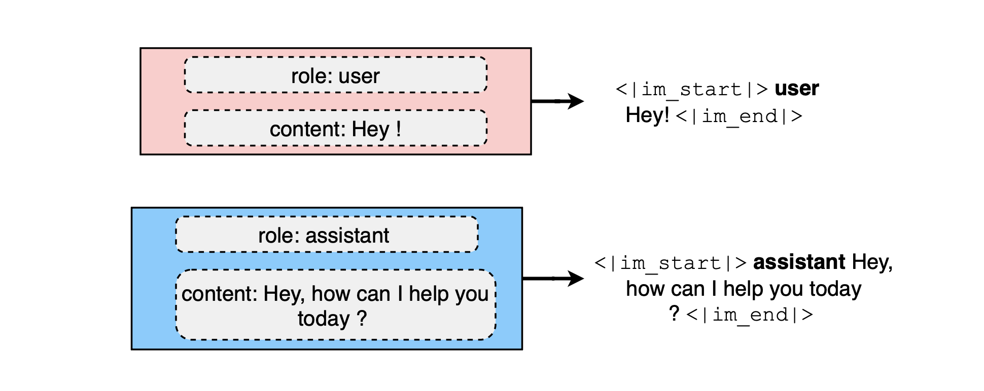
When using LLMs, you typically send a set of input messages, each with a role and content. This is because during fine-tuning, the model continue training on multi-turn dialogue data where additional special tokens are introduced to guide generation. A chat template is typically applied before passing the resulting text to the tokenizer, which produces the tokens that are then processed by the LLM until the next token is predicted. The same applies to an agent's conversation history.
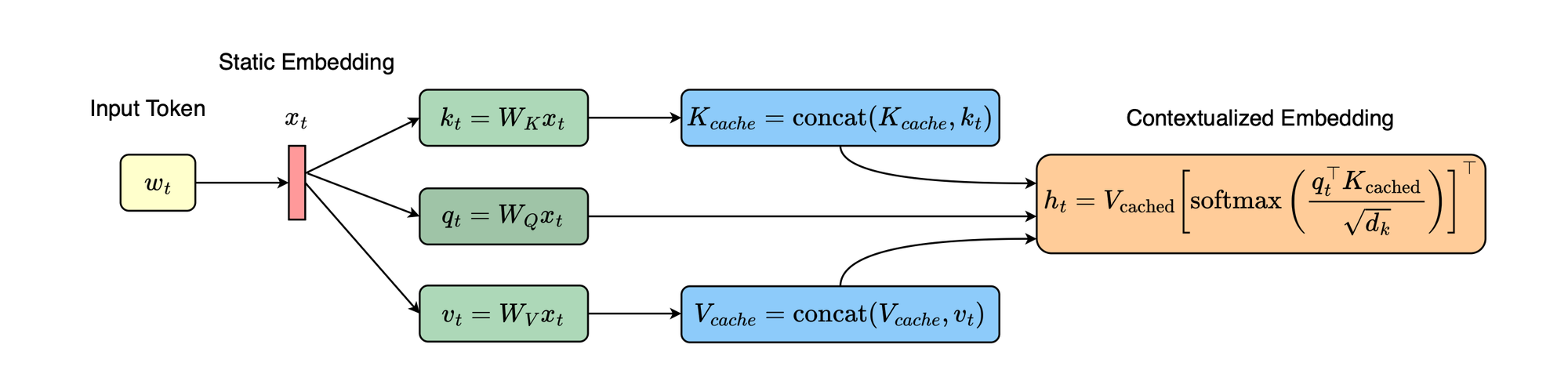
To reduce the cost associated with repeatedly computing unchanged token representations. specifically the keys and values for each Transformer block, the KV cache is used to cache the keys and values of previous tokens thereby reducing redundant computation. Assuming the corresponding prefix has not changed, such as a system prompt containing tool descriptions, the next token can attend to the cached keys and values rather than recomputing them, and generation continues in an autoregressive fashion.
That is all. I tried to keep this post short. If you are interested in learning more technically, including how LLMs are trained, take a look at my updated notes: https://books.deep-kondah.com which now includes the LLM part (it is in draft, the final reviewed release is planned for December 2026 once GPUs, inference engines and more code/training sections are included).
As promised, the next post and part will be about CUDA/GPU Programming followed by inference engines (vLLM, TensorRT, llama.cpp).