The goal of this post is to explain how vector similarity search works internally. Why is this interesting? Because Retrieval-Augmented Generation or RAG is typically implemented using vector search over text embeddings. Embeddings are basically a bottleneck that compresses the semantics of a paragraph or chunk into a continuous

The goal of this post is to explain how vector similarity search works internally. Why is this interesting? Because Retrieval-Augmented Generation or RAG is typically implemented using vector search over text embeddings.
Embeddings are basically a bottleneck that compresses the semantics of a paragraph or chunk into a continuous vector representation, which can then be used for various downstream tasks, including similarity search and classification.
In a vector-based RAG pipeline, documents are first split into chunks (because the context window feeding large models is limited). Each chunk is then embedded into a high-dimensional dense vector representation, and the resulting vectors, together with their associated metadata, are indexed in a vector database such as postgres/pgvector. At inference time, the user query is embedded into the same vector space, and the system retrieves the nearest chunks, typically using Approximate Nearest Neighbor or ANN search, optionally followed by a reranking. The retrieved context is then passed to the LLM to generate grounded responses. Hybrid and graph-based RAG systems also rely on vector search, for example to identify seed nodes before graph expansion.
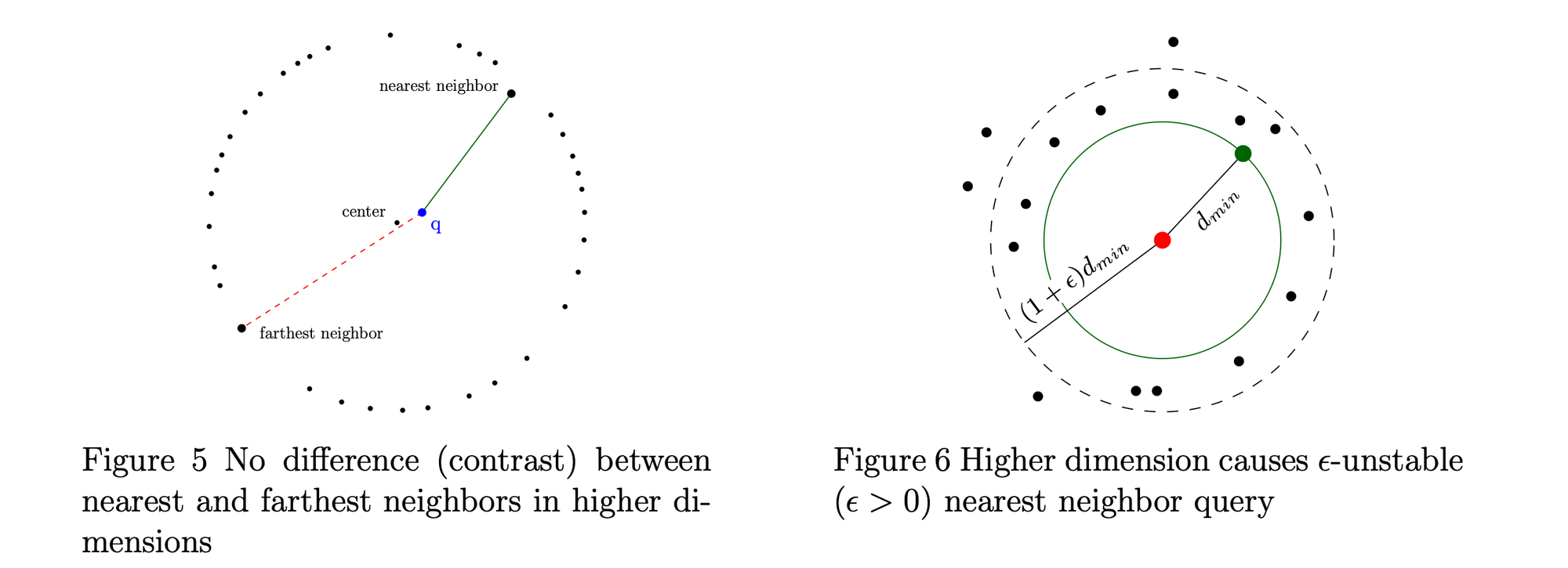
But wait, if embeddings live in high-dimensional spaces, should we worry about the curse of dimensionality [1]? In high-dimensional spaces, distances can become less discriminative: the contrast between the nearest and farthest points may shrink, making points appear almost equidistant.
So why does vector-based RAG work at all?
In this post, we explain how vector search operates, including SOTAs Approximate Nearest Neighbor ANN indexing methods, why text embedding models are more robust to the curse of dimensionality, and when Graph-RAG can provide a better retrieval alternative; for example, when relationships, multi-hop reasoning, entities, provenance, or structured context become important.
I will keep this post relatively short. If you are interested in a deeper analysis, I am sharing a draft of technical notes, including an analysis of the FAISS implementation [8]; it consolidate many of the key ideas discussed here and should provide a more complete understanding of how vector search works in practice.
Given a query vector \(q\), the \(k\)NN, or \(k\)-nearest neighbor, search involves identifying the \(k\) closest data points in a vector database. Solving the \(k\)NN search consists of computing the distance between the query and a set of candidates, which could be the whole dataset.
If we assume that the dimension of the vector space is \(d\), computing the squared Euclidean distance with each vector in the database can be prohibitively expensive. Using the squared distance does not change the ranking, since the square function is increasing on \(\mathbb{R}_{+}\), where distances are positive.
Computing the distance to one vector requires \(O(d)\) floating-point operations, or FLOPs, and computing distances to all \(N\) data points requires \(O(Nd)\) operations. When both \(d\) and \(N\) are large, we cannot generally expect a real-time response, for instance when integrating \(k\)NN search into RAG, which has real-time constraints.
This is why most solutions use approximate \(k\)NN search, trading some accuracy for speed. Most of the solutions covered later restrict the set of candidates, compute distances only for those candidates, and maintain a mini/max-heap of size \(k\) while navigating the euclidean space. The heap is queried and updated whenever the current candidate is better than the current threshold, i.e., when it is closer than the worst candidate currently in the heap. Finally, the algorithm returns the best \(k\) nearest-neighbor results.
We will discuss later how to produce a representation where variance, or energy, is concentrated in the leading dimensions, with less energy left in the residual dimensions; this enables faster pruning and reduces the cost of distance computation at runtime.
In high-dimensional spaces, data samples tend to be sparse. For example, if we consider a ball centered at a point, it will contain very few data points. This sparsity makes generalization harder, because covering the ambient space requires an exponentially growing amount of data.
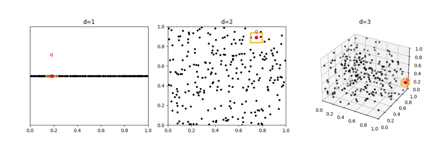
The curse of dimensionality also affects nearest-neighbor search. As the dimensionality of the ambient space increases, nearest neighbor search becomes less meaningful due to distance concentration; the ratio \( d_{\max} / d_{\min} \) converges to 1, where the \(d_{\max}\) and \(d_{\min} \) refer to the maximum and minimum distances achieved between a query vector and the dataset; meaning the distances to the nearest and farthest neighbors become nearly identical (e.g., under Minkowski distances, assuming IID data [2]).
At first glance, the above seems problematic for vector-based RAG., especially since embedding dimensions can be large (e.g., 1536 dimensions for some models [3]). If distances become unreliable in high dimensions, then vector search itself might appear fragile right ?. As shown below, when dimensionality increases, the standard deviation of distances decreases, illustrating distance concentration.
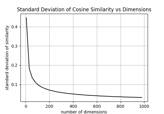
While random vectors in high-dimensional spaces tend to become nearly orthogonal:
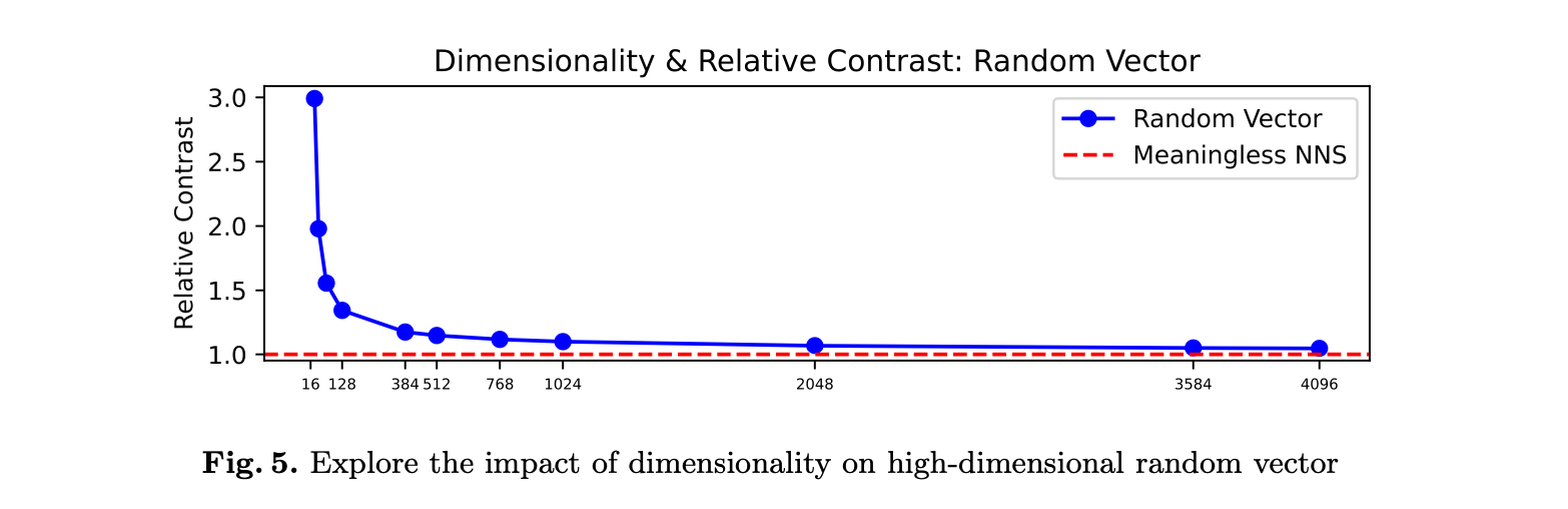
real-world data are not uniformly and/or randomly distributed.
Embedding spaces exhibit structure and their dimensions are not independent (e.g removing randomly 50% of embedding dimensions results in only a minor drop in performance [5]). In other words, the intrinsic dimension of the data is much lower than the ambient dimension.
Because of correlations between dimensions, embeddings are more robust to increases in dimensionality compared to purely random vectors [4]. A relatively large ratio between \( d_{\max} \) and \( d_{\min} \) and low intrinsic dimensionality, reduces or mitigates the impact of the curse of dimensionality.
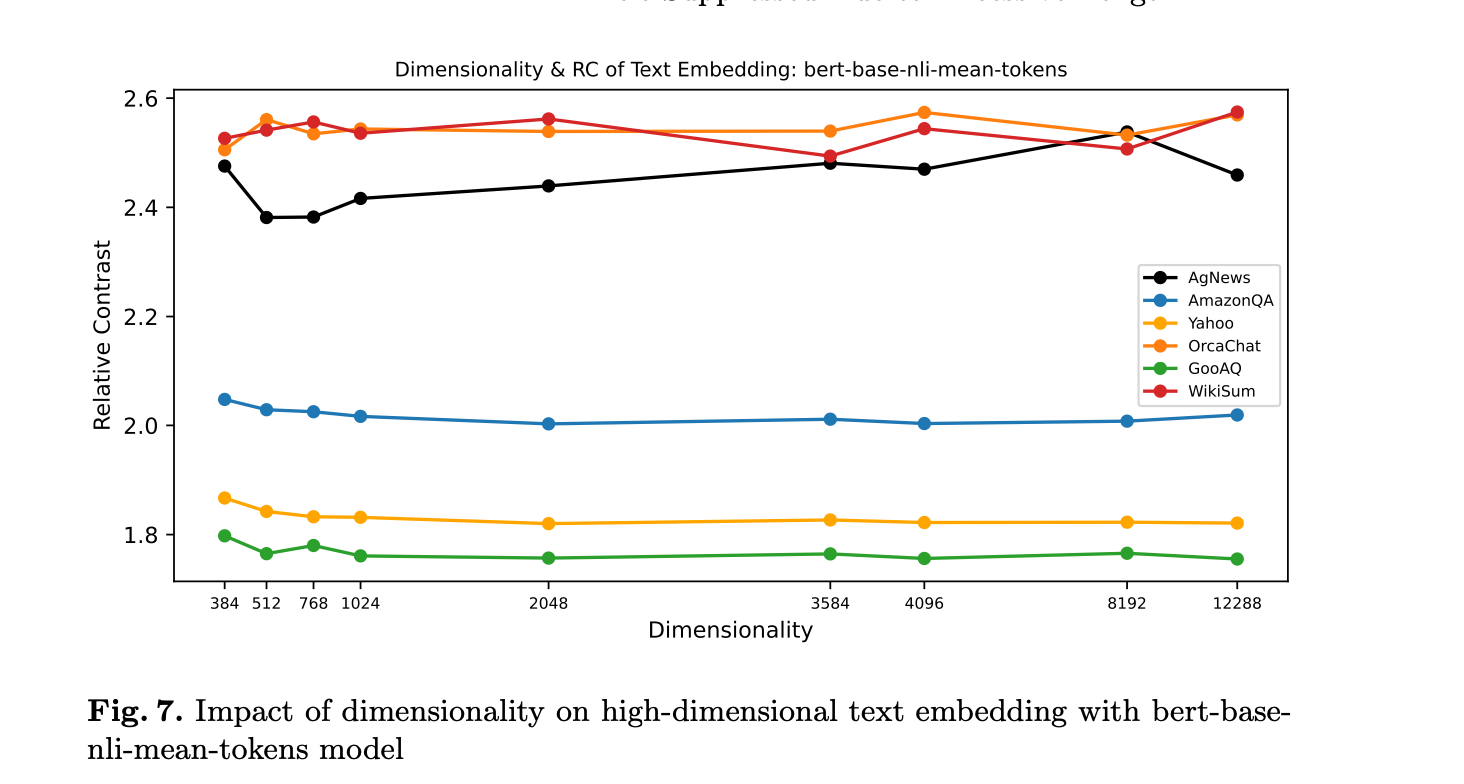
The curse of dimensionality is not limited to nearest-neighbor search. It also affects classifiers, since sparsity makes it harder to generalize across the ambient space. High dimensionality also increases storage and computational cost. For example, computing an inner product between two vectors of dimension \(d\) requires \(d\) fused multiply-add operations. For \(N\) vectors, exhaustive search therefore costs \(O(Nd)\), or approximately \(O(N)\) when \(d\) is fixed and much smaller than \(N\).
One common mitigation strategy is dimensionality reduction, where data is mapped to a lower-dimensional space while preserving important directions (e.g PCA) [6].
The first and most naive implementation of vector search is brute-force \(k\)-nearest-neighbor search over the entire dataset. In this case, when \(N\) is large, search can become very slow, since most of the runtime is spent computing distances, such as squared \(L_2\) distance, between the query vector and all vectors in the database.
This type of index is often a good starting point when experimenting with a small dataset, because it is simple and exact. However, once the dataset becomes large, exhaustive search becomes expensive, and approximate \(k\)-nearest-neighbor methods are usually next steps.
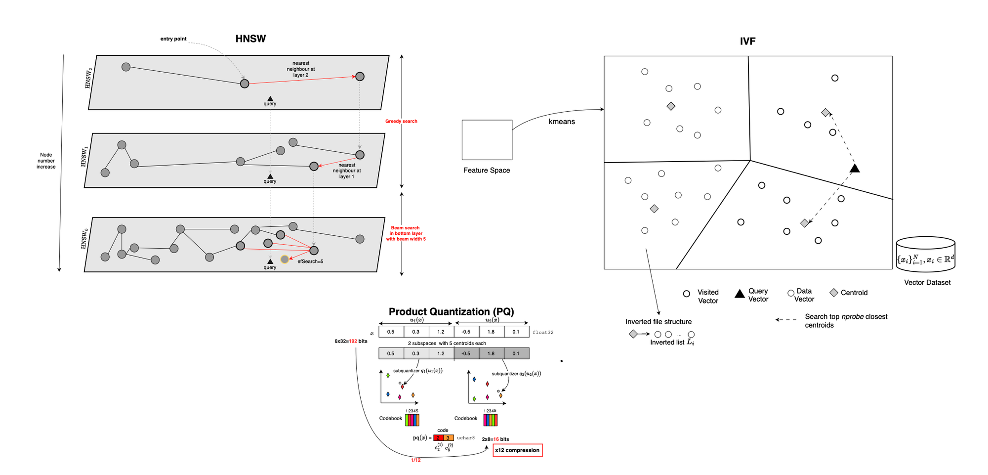
The idea behind IVFFlat [9], or inverted file indexing, is to partition the vector space into clusters or regions. Instead of searching through the entire Euclidean space point by point, the search is restricted to the nearest clusters or cells.
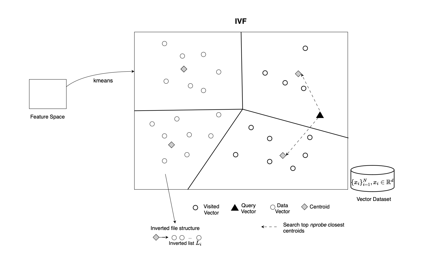
During training, a clustering algorithm typically \(k\)-means is used to learn a set of centroids. Each centroid is associated with a list of vectors that belong to its cluster.
At query time, the query vector \(q\) is compared with the centroids, and only the closest clusters are selected. The vectors inside these selected clusters become the candidate set. The exact distances between \(q\) and the candidate vectors are then computed, and the \(k\) nearest neighbors are returned, typically maintaining the current best results using a heap.
The trade-off is controlled by the number of clusters searched. Searching more clusters improves recall but increases latency, while searching fewer clusters improves speed but may miss relevant neighbors.
So, there are basically two parameters, nlist is the number of centroids or clusters, and nprobe, the number of regions that are visited at query time.
IVFPQ [10] combines inverted file indexing with product quantization, or PQ, to reduce memory and storage requirements.
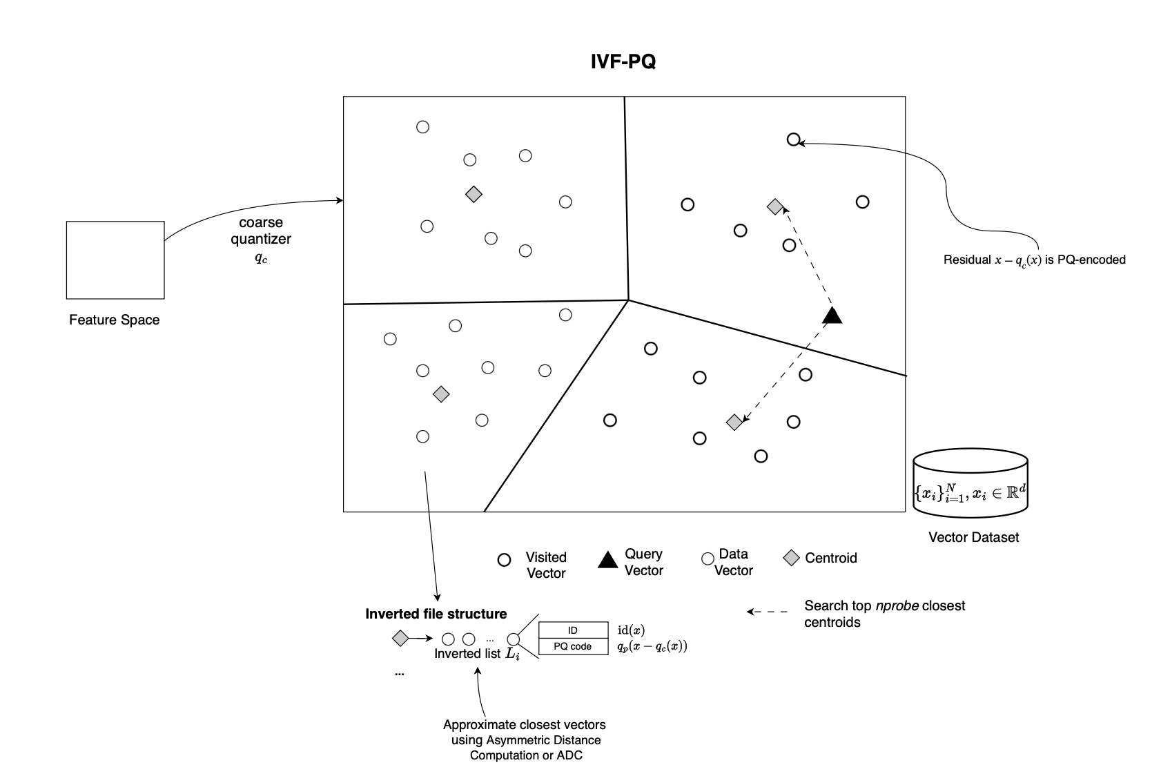
As in IVFFlat, a coarse quantizer is first trained, using \(k\)-means, to partition the vector space into clusters. Each database vector is assigned to one of these coarse clusters. However, instead of storing the full vector, IVFPQ compresses each vector using Product Quantization or PQ.
In PQ, each vector is split into multiple subvectors. For each subvector space, \(k\)-means is applied separately to learn a set of subcentroids, also called a subcodebook. Each subvector is then represented by the identifier of its nearest subcentroid. Therefore, what is stored in the index is not the full floating-point vector, but a compact code made of subcentroid identifiers.
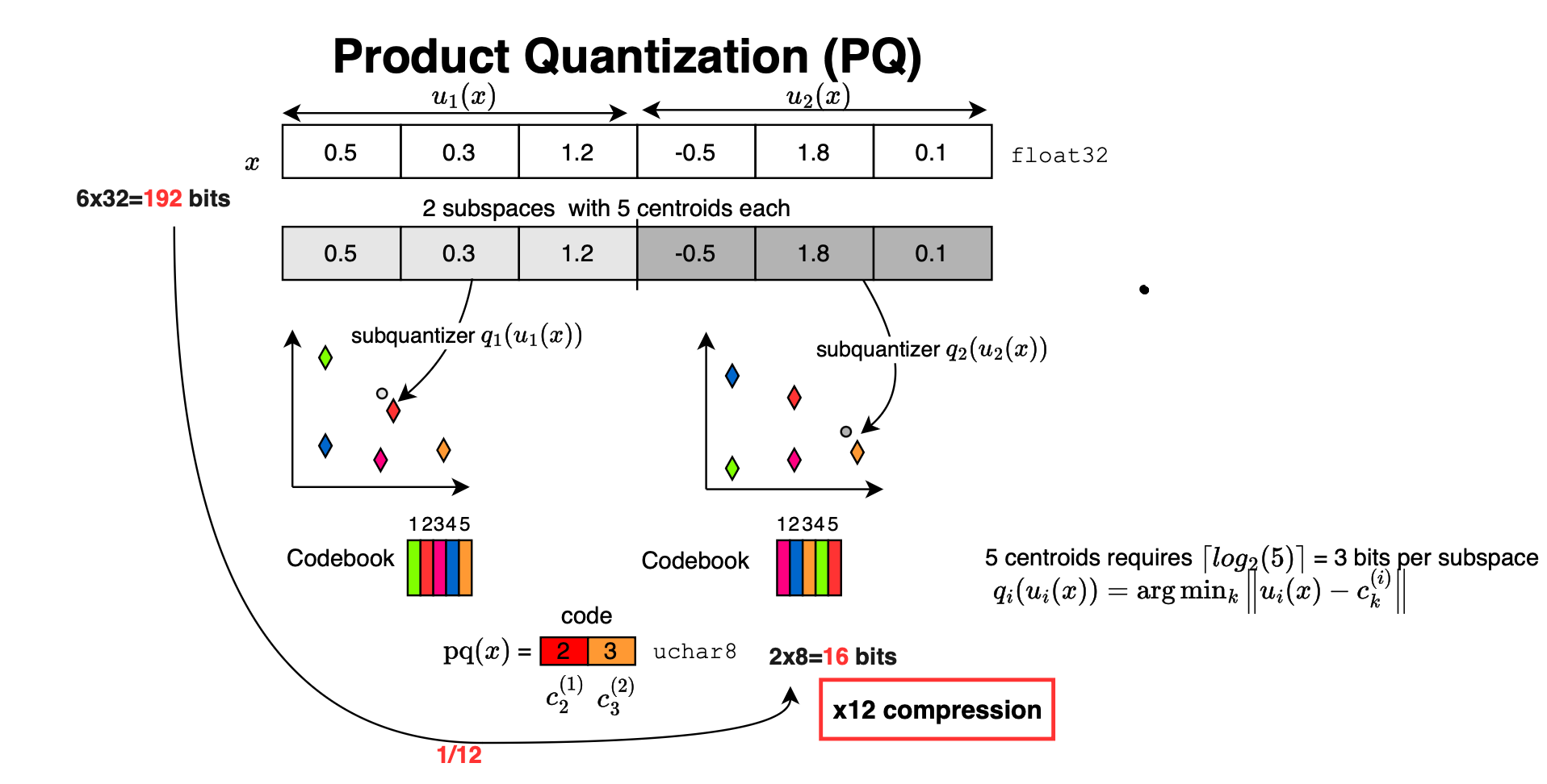
At query time, the coarse quantizer is first used to select the most relevant clusters. Then, distances between the query and the PQ-encoded candidate vectors are approximated using the learned codebooks thereby trading some approximation error for speed and efficiency.
For more implementation details, see my technical notes.
HNSW[11], or Hierarchical Navigable Small World graphs, is very different from IVF-based methods. Instead of partitioning the vector space into clusters, HNSW represents vectors as nodes in a graph.
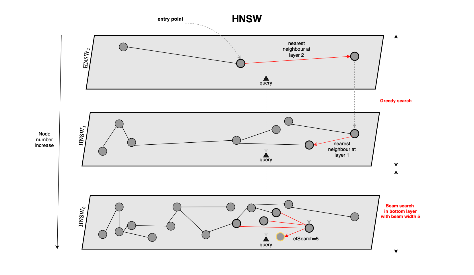
More specifically, HNSW builds a multi-layer graph. During indexing, each inserted vector is assigned a maximum layer. Higher layers are sampled with exponentially decreasing probability, meaning that only a small number of points appear in the top layers. These upper layers contain fewer nodes and provide long-range connections, while the lower layers are denser and contain more local neighborhood information.
When a new vector is inserted, the algorithm starts from an entry point in the highest available layer and performs greedy search to find good neighbors. The new node is then connected to selected neighboring nodes layer by layer, down to the base layer.
At query time, search also starts from the upper layers. A greedy search is first applied on the sparse top layers to quickly move toward a promising region of the graph. Once the search reaches the bottom layer, a wider beam-search-like procedure explores neighboring nodes. Candidate queues are used to manage nodes to visit, while a heap maintains the current best nearest-neighbor results.
For more implementation details, see my technical notes.
Panorama [7] was introduced recently to accelerate distance computation over candidate vectors, which is often the dominant part of runtime [6].
The main idea behind Panorama is to avoid computing distances over all dimensions whenever possible. Instead of always paying the full cost \(O(dN)\), where \(d\) is the embedding dimension and \(N\) is the number of candidate vectors, Panorama aims to reduce the effective dimensional cost to something closer to \(O((d / \alpha)N)\), for some acceleration factor \(\alpha\).

Specifically, panorama uses PCA and gradient-descent to learn an orthogonal transformation. The mapping maps vectors into a new representation that compacts the signal’s energy into the leading dimensions thereby enabling pruning using distance lower and upper bounds.

During search, these bounds allow to discard some candidates without evaluating the full-dimensional distance, thereby reducing the overall cost of candidate distance computation.
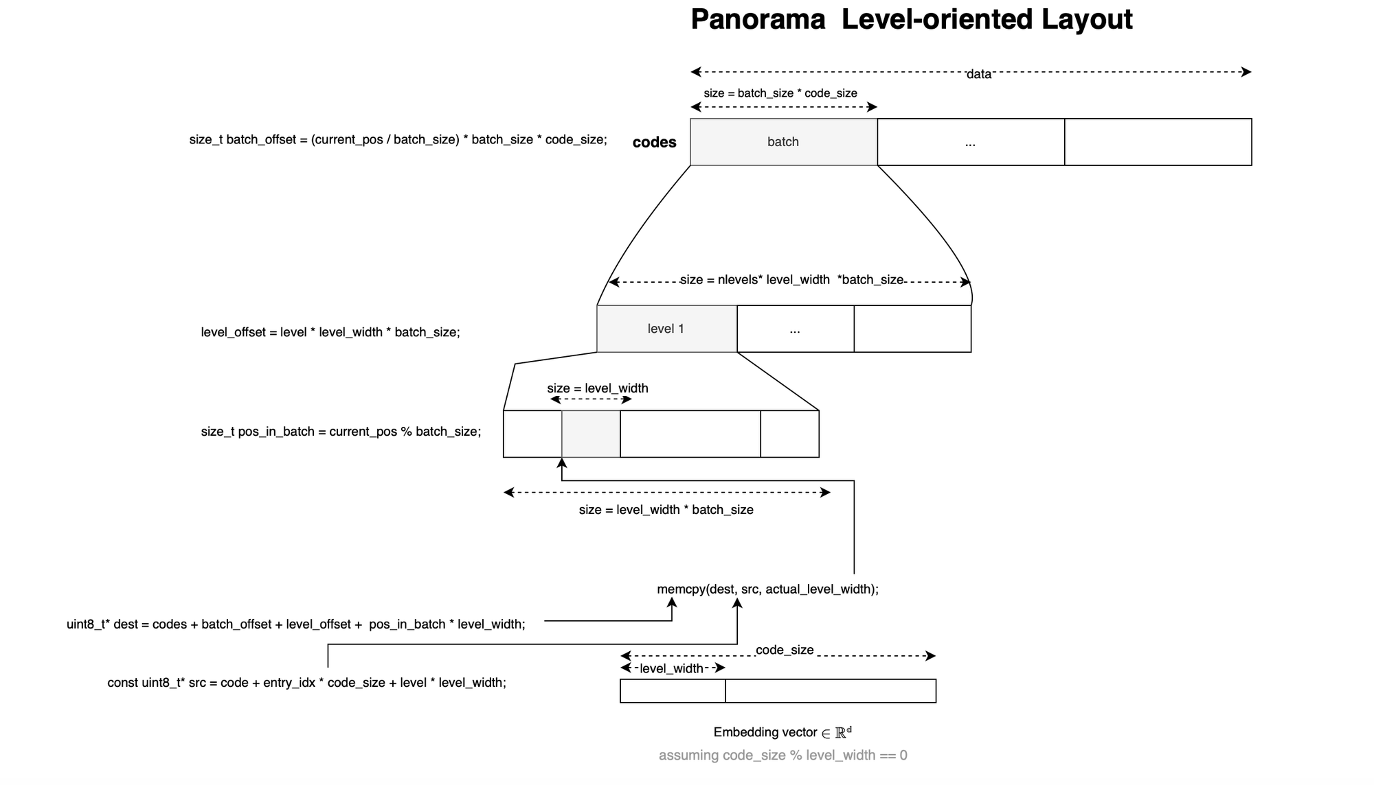
If we look at the FAISS implementation, a level-major layout is used in order to reduce memory traffic and increase locality:
When the documents stored in a vector database contain explicit structural information, the underlying data may be naturally representable as a graph. For example, a cyber threat intelligence report may describe a threat campaign, the threat actor behind it, the malware they deploy, and the files they drop, including filenames, hashes, and other indicators of compromise. These entities and their relationships form a natural knowledge graph.
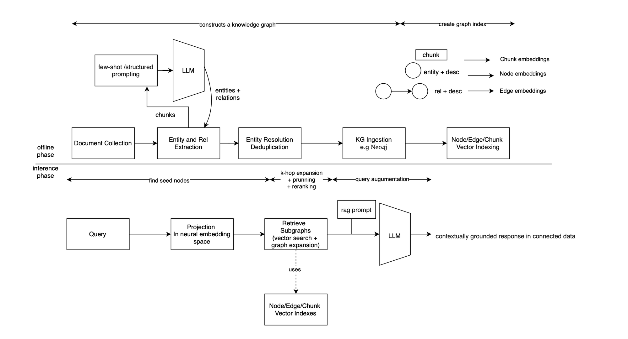
However, standard chunking procedures tend to disrupt these relationships. By fragmenting documents into isolated chunks, semantically linked elements may be separated across different pieces of text. As a result, the retrieval process may need to recover multiple disjoint chunks that were originally part of the same coherent structure. This can lead to a loss of relational context and increased retrieval overhead.
This becomes especially important when considering provenance graphs. In security applications, one may want to fuse a CTI graph with a provenance graph to support deeper attack detection, correlation, and investigation. Vanilla vector-based RAG pipelines are not well-suited for preserving or leveraging these structured dependencies, because they primarily retrieve text chunks based on semantic similarity rather than explicit relationships i.e substructure.
Graph-based RAG addresses this gap. The core idea is to process documents in order to extract entities and relationships, represent those relationships as edges, and construct a graph-based representation of the underlying knowledge. The resulting graph can then be indexed and queried using graph embeddings, such as node, edge, or subgraph embeddings, with or without graph neural networks or GNNs; which support efficient retrieval, anchor-node selection, and graph traversal.
The above preserves structural semantics and enables relational reasoning during retrieval. It can also reduce redundancy, since duplicate entities can be identified and merged more naturally in a graph. In addition, graph-based retrieval can lower retrieval cost by using structured navigation instead of broad semantic search over many independent chunks. It can also improve fact-level retrieval and unlock behavior modeling, particularly in security contexts where relationships between entities, events, and artifacts are critical.
To better understand how GraphRAG is implemented in practice, see my technical notes, where I cover the LightRAG implementation [12].
If you read my posts regularly, you know that I include security in everything I do.
When you implement RAG, you must understand that the semantics of the user input guide the retrieval process. If an adversary inputs something sensitive, such as incident report tags or similar terms, and the underlying database does not enforce document-level access control, the attacker could access documents they should not be able to access; because they would be returned as most similar documents or chunks.
So, do not expect users to use the system in a semantically correct or intended way. This is one of the main attack vectors when implementing RAG (of course you also have document poisoning and prompt injection...).
If we look at CVE-2026-3357[13], it is basically a defect in IBM Langflow Desktop, a deserialization flaw resulting from an insecure default in the integration of the FAISS component for RAG. A Pickle file, used by FAISS for loading vector index files, enables Langflow workflows where users can load vector store indexes to support semantic search within an LLM pipeline. If a malicious Pickle file is loaded on user demand, it could lead to arbitrary code execution.
[1] https://en.wikipedia.org/wiki/Curse_of_dimensionality
[2] https://arxiv.org/pdf/2401.00422
[3] https://developers.openai.com/api/docs/guides/embeddings
[4] https://arxiv.org/pdf/2410.05752
[5] https://arxiv.org/html/2508.17744v1
[6] https://arxiv.org/pdf/2404.16322
[7] https://arxiv.org/pdf/2510.00566
[8] https://github.com/facebookresearch/faiss
[9] https://arxiv.org/pdf/2401.08281
[10] https://pubmed.ncbi.nlm.nih.gov/21088323/
[11] https://arxiv.org/pdf/1603.09320
[12] https://github.com/hkuds/lightrag
[13] https://nvd.nist.gov/vuln/detail/CVE-2026-3357