Large Models Training

The urge to train expansive deep learning models, particularly large language models, is ever-growing. A single GPU often falls short in providing the required memory capacity to accommodate various parameters and data, thus necessitating the employment of multiple GPUs. Additionally, the time cost of training complex models can be daunting. Speeding up the training process reduces the indefinite wait times, making model development more feasible and efficient.

Pre-reading Requirements

I assume readers have at least a basic background in Machine Learning (understanding concepts such as probability, embedding space, training vs. testing, etc.).

Summary

• As Large Language Models (LLMs) continue to increase in size, the research community is actively seeking efficient algorithms for training these models. A widely utilized concept in Machine Learning to enhance training efficiency is parallelism, which involves leveraging multiple nodes to speed up the process.
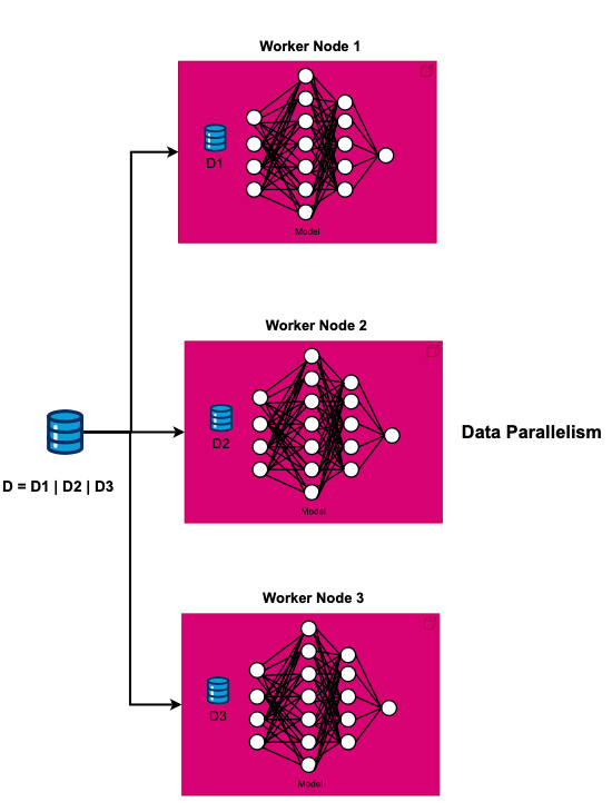
• One prevalent approach to distributed Deep Neural Network (DNN) training is Data Parallelism (DP). In DP, the model's weights are replicated across numerous nodes. Each node processes a unique subset of data simultaneously. Upon completion, all nodes collectively contribute to updating the overall gradient.
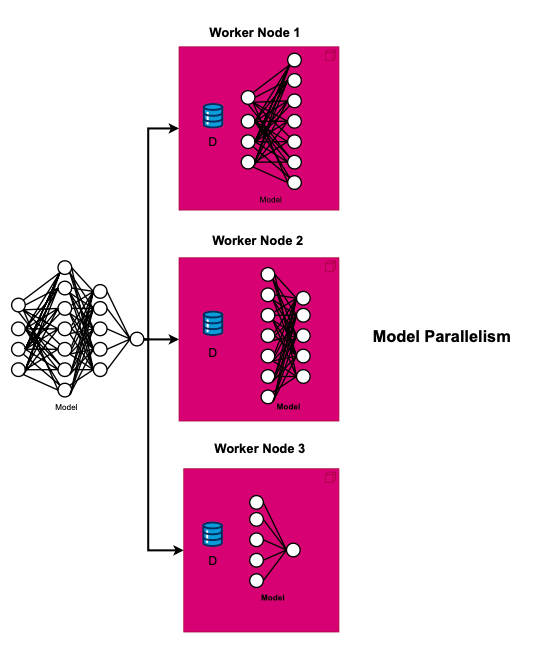
• Model Parallelism (MP) becomes crucial when a model's size exceeds the capacity of a single device. In contrast to DP, where each device holds a complete model copy, MP assigns only a segment of the model to each device. This approach conserves memory and accelerates computations.
• Expert Parallelism (EP) involves distributing model subnetworks (experts) across a pool of devices, thereby alleviating the memory and computational loads on individual devices.

Stochastic gradient descent (SGD)

In machine learning, the principle of empirical risk minimization (ERM) refers to the methodology used to approximate an arbitrary function (or hypothesis) f, based on available data, X. Given that our function f is defined by a set of parameters, the primary objective is to tune these parameters to minimize the empirical loss.

Empirical loss is defined as the difference between the predictions made by f and the actual data in X. To achieve the optimization task of minimizing the empirical loss, various optimization algorithms are employed to find the best parameters that fits the training set well.

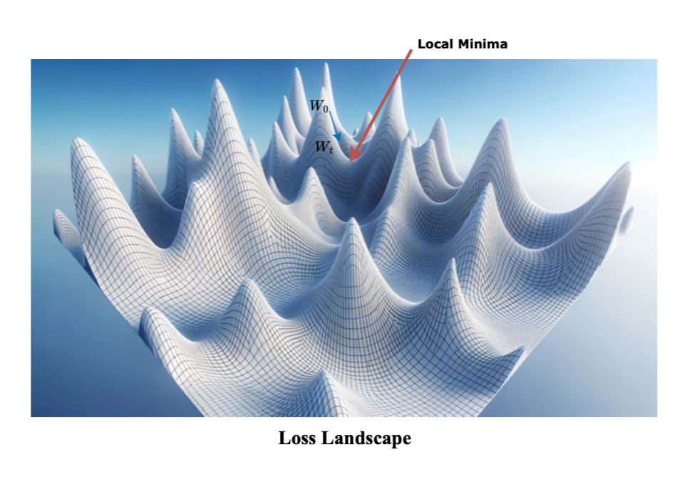
Gradient descent (GD) is one of the most known and used optimization algorithm for minimization. The process entails navigating through the parameter space, starting from an initial point, in a descent direction that leads to a decrease in the loss function. The resulting updated parameters or weights represent the new learned values. The direction of descent can be determined by calculating the gradient, which provides the steepest descent direction, so we update the parameters in the opposite direction.

A learning rate or step size is applied to control the size of each step taken during the optimization process. Often, a step size policy is utilized to ensure convergence and facilitate stopping at an optimal point. Although a constant learning rate can also be used, it is common to adopt a policy-based approach.

Additionally, It is possible to encounter situations where the gradient vanishes at a certain point in the parameter space. This occurrence indicates that the model has reached a stationary point, where further learning becomes challenging as there is no clear direction to proceed (your model stops learning/advancing). Smooth and convex loss functions are desirable in this case as they increase the likelihood of successful optimization, while non-convex functions may lead to overfitting.

Here's the algorithm for GD:

$$
\theta = \theta - \eta \cdot \frac{1}{n} \sum_{x_i, y_i \in D} \nabla_{\theta} L(\theta; x_i, y_i)
$$

θ is the vector of parameters, η is the learning rate, n is the number of training examples in dataset D, L(θ; xi, yi) is the loss function calculated on the ith training example (xi, yi), and ∇L(θ; xi, yi) is the gradient of the cost function with respect to the parameters θ.

SGD (in short for Stochastic Gradient Descent) is a variant of gradient descent that mitigates the computational burden associated with computing the gradient over the entire dataset (where one would need to calculate the gradient for each data point and then average them). SGD and its derivates are the most used optimization algorithms for solving complex problems with nonconvex loss functions.

Instead of using the full dataset, SGD first shuffles the dataset and then divides it into batches. At each iteration, it selects a batch of training data to compute the gradient and update the model parameters. Sampling batches from the datset can be either with replacement or without replacement. The term Mini-Batch SGD is often used to denote the approach where a mini-batch is used to approximate the gradient, while using just one sample for the gradient computation is also sometimes referred to as SGD. For simplicity, in this context, we'll use SGD to denote the mini-batch variant.

The algorithm for SGD is almost similar to vanilla GD, the difference lies in how the average is calculated:

$$
\theta = \theta - \eta \cdot \frac{1}{b} \sum_{x_i, y_i \in B} \nabla_{\theta} L(\theta; x_i, y_i)
$$

Here the batch of the current iteration is B of size b << n.
The introduction of randomness in SGD gives rise to the term "stochastic" since the selected training examples varies. By using this random sampling approach, SGD reduces the computational burden, enabling faster iterations compared to traditional GD. However, this comes at the cost of a lower convergence rate, as the noisy estimates of the gradient introduce fluctuations in the optimization process. Additionally, achieving convergence in GD does not guarantee convergence in SGD, as SGD only considers a subset of data points for averaging instead of the entire dataset.

Since SGD relies on a small subset of the training data, its gradient estimates can be noisy, leading to erratic movement in the weight space. The noisy updates can sometimes make the training unstable, especially with large learning rates.

Momentum is a technique that takes into account the previous gradient steps to smooth out updates. It helps to accelerate convergence and dampen oscillations.

A static learning rate might be too large during some stages of training, causing divergence or oscillation, and too small during others, leading to slow convergence. Algorithms like AdaGrad, RMSProp, and Adam adjust the learning rate based on the history of gradients. This allows the model to have larger updates in sparser regions and smaller updates in denser regions, leading to more efficient training.

Finally, As neural networks become deeper, gradients can grow exponentially (explode) or diminish to near-zero values (vanish) as they are back-propagated. This makes training deep networks challenging. Techniques like Batch Normalization aim to mitigate these issues by normalizing intermediate layer activations. This helps maintain a steady distribution of activations, making training more stable and often faster.

Data Parallelism (DP)

One of the most popular distributed DNN training approach is Data Parallelism (DP). DP means copying model weights to many nodes. Each node gets a different piece of data to process at the same time. After all the nodes completes, they contribute to the update the overall gradient. There are several approaches to data parallelism including Parameter Server (PS), All-Reduce, and Gossip, which we will cover later.

Specifically, in mini-batch SGD, each node i gets a data distribution Di. We define the local loss Li as:

$$
L_i(\theta) = \mathbb{E}_{d \sim D_i}[L(\theta, d)]
$$

The update rule of SGD is defined then as:

$$
\theta_{t+1} = \theta_{t} - \frac{\gamma_t}{N} \sum_{ i \in \text{workers}} \nabla_{\theta} L_{i}(\theta_t)
$$

Where γt is the learning rate. The models are deployed across all devices and uses the same initialization parameters, this means that all the models house a consistent version of the model (at any time).

From the formula above, we see the all the workers collaboratively contribute to finding the best possible value for θ by giving their computed gradient ∇Li(θ), after receiving the gradients, the model parameters are updated and broadcasted to all workers, which introduces communication costs and limits the system scaling efficiency.

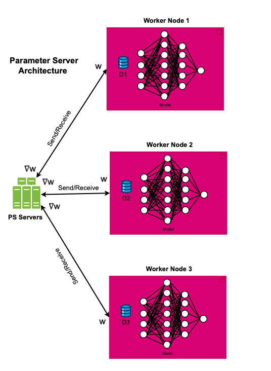
Parameter Server (PS)

Data parallelism can be achieved using the Parameter Server (PS) model, where worker nodes send their computed gradients to the PS. The PS, which usually runs on a CPU, aggregates these gradients, updates the model parameters and then sends the updated parameters back to all worker nodes.

One issue with PS centralized architecture is the the communication overhead, the PS needs to communicate with all the worker nodes, thus creating a communication bottleneck.

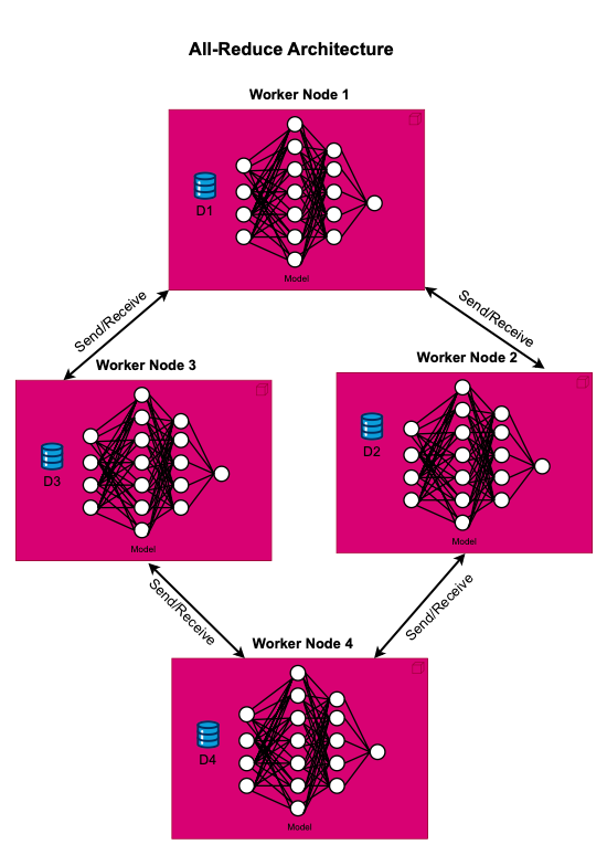
All-Reduce

To mitigate the communication bottleneck associated with the Parameter Server (PS) model, All-Reduce architecture has been adopted, which distribute the communication workload among the workers and allows for gradient aggregation without the need for a central server to orchestrate the communication. Among the All-Reduce algorithms, the ring-based approach is notably popular. Furthermore, the All-Reduce primitive is often optimized to achieve high performance with reduced communication overhead.

Bulk Synchronous Parallel (BSP)

In Bulk Synchronous Parallel (BSP) scheme, every node does a batch of work, and only when all the working nodes have finished the respective calculations, the model gets updated. One advantage in contrast to async update is no stale gradient is used as the each node stops by a synchronization barrier from training the next iteration until global model receives all results of other active workers. However, gradients sychronization overhead can be a major factor preventing linear scalability. Some nodes may be faster than others which leads to the straggler or slowest worker problem. Additionally, the aggregation of all gradients leads to high communication costs.

Asynchronous Parallel (ASP)

In asynchronous scheduling, when a subset of nodes finishes, the model is updated right away without waiting for the others, and the result is broadcasted to the nodes that have completed their communication without the barrier of waiting for slower workers. As a result, different nodes or GPUs might be working with slightly different versions of the model at any given time. Asynchronous updates (supported by PS - with All-Reduce it is not easy) can lead to faster training times because there's no waiting involved, effectively eliminating the problem of stragglers. However, it can also introduce instability into the training process, as the model updates can become more erratic. Some slower workers will contribute delayed or stale gradient updates to the globally shared weights. This is why synchronous SGD remains the state-of-the-art nowadays.

Stale Synchronous Parallel (SSP)

Stale-Synchronous Parallel (SSP) is a relaxation of the Synchronous Parallel model that mitigates the straggler problem. You can think of it as a conditional asynchronous update that places a bound on the staleness (SSP = BSP + ASP). In this scheme, faster nodes get the chance to pull new model parameters using stale gradients and proceed with computation. However, a synchronization barrier is enforced when the gap between faster and slower nodes exceeds a certain threshold. This reduces inconsistency and promotes convergence.

Gossip SGD

In the gossip scheme, there is no global model updates and no need for a collective communication. Each node or worker houses its own model, on which, it effectuates the learning by talking to its neighbors, that is, each node averages only with its neighbors.

In the gossip, each node does not have to communicate with all the nodes but only a random subset, this means at each step you would get a different partner. This makes Gossip attractive from a failure-tolerance perspective.

During training, the algorithm does not guarantee parameter consistency across all workers after each communication, but guarantees it at the end of the algorithm (i.e., consensus). Gossip protocol based approaches are much faster than PS and All-Reduce but may suffer from slower convergence rate.

As discussed, several approaches have been proposed to implement Data Parallelism. These strategies aim to utilize bandwidth resources more efficiently while ensuring the convergence property is maintained. A primary issue with DP is that every GPU retains a full copy of the model, leading to potential inefficiencies. To address this, strategies such as intermittently offloading parameters to CPU memory have been suggested. Additionally, the All-Reduce primitive could pose a scalability challenge.

Model Parallelism (MP)

Model Parallelism (MP) comes into play when a model is too big to fit in one device. Instead of every device having a full copy of the model like in DP, in MP each device gets just a part of it. This saves memory and speeds up calculations. Examples of this are the ways GShard handles the MoE (in short for Mixture of Experts) Transformer and how the Switch Transformer works, making things more efficient and scalable.

While MP reduces the memory requirements and efficiency it may incurs additional communication between layers, an all-to-all communication is, in fact, required.