Scaling Large Language Models

In recent years, there has been a consistent trend in the expansion of the dimensions of large language models. They’re being trained on ever-increasing amounts of data and displaying ever-improving performance.

However, is this growth merely for the sake of expansion, or is there a deeper rationale behind their increasing magnitude? Does the impressive performance directly correlate with their size?

In this article, we aim to illuminate these questions, providing a comprehensive understanding of why larger language models trained on vast corpora excel. We will also delve into how companies like Google, OpenAI and Meta optimize parameters to ensure computational resources are optimally used and predict the performance of trained models.

Intuitively, one might assume that increasing both the model size and the training data would enhance the model’s performance. However, substantiating this intuition with theoretical or empirical studies presents a challenge. This is because training neural networks is not always stable, and different training mechanisms can yield different results. So, it is not straightforward an should be done carefully.

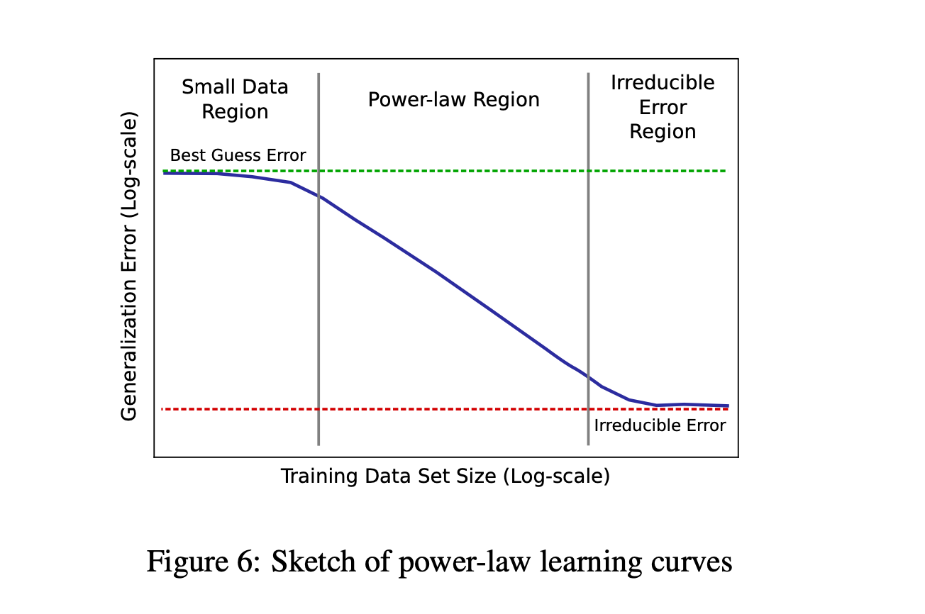
Deep Learning Scaling is predictable, empirically is one of the first research papers that empirically illuminated the relationship between training set size, model size, and model performance across various application domains and models, even before the emergence of large language models. The research demonstrated the presence of power-law learning curves across several domains. Even though different applications produce distinct power-law exponents and intercepts, these learning curves are consistent across a wide spectrum of models, optimizers, regularizers, and loss functions.

Pre-reading Requirements

This article assumes that readers have a basic understanding of Machine Learning, Deep Learning and Large Language Models (LLMs).

Summary:

• The Scaling Law provides a way for predicting the performance of models in advance.
• With a fixed computational budget for training, Scaling Law can guide you to the optimal number of training dataset (tokens for LLMs) and the appropriate number of parameters to use for effective performance.
• Scaling Laws are instrumental in conserving resources, as searching for hyperparameters becomes impractical when pretraining LLMs, you often only get one shot to get it right. They assist in answering questions like, "With my available compute for training, should I increase the amount of data, the number of tokens, or both simultaneously?". Moreover, it can guide you to the optimal batch size and number of steps necessary for updating the model's parameters.
• While specific architectural details (e.g., depth, width) are important, the Scaling Law suggests that the data, the number of parameters and the amount of compute typically have a greater impact on model performance. Hence, the focus should be on the efficient utilization of data for training LLMs.
• As the availability of data eventually caps, simply increasing the number of parameters without sufficient data will lead to diminishing returns, making further resource investments inefficient. It is, therefore, critical to manage how data is used and to train models efficiently to avoid hitting a plateau in performance where additional resources no longer yield significant improvements.
• The Scaling Law does not provide an exact prediction of performance; instead, it offers a rough estimate.
• One should exercise caution with empirical conclusions. They warrant further
  validation, especially theoretical proofs, as varied training strategies might yield diverse results.

Has Moore's Law Reached Its End?

Moore's Law, as posited by Gordon Moore, co-founder of Fairchild Semiconductor and Intel, asserts that the number of transistors that can be placed inexpensively on a computer chip doubles approximately every two years. As the years have passed, this observation has largely proven accurate. However, we are now approaching the limits of the physical capacity a chip can accommodate. This indicates that manufacturers may struggle to maintain the same rate of advancement in CPU and GPU capabilities, at least not without incurring higher costs.

For instance, in September 2022, Nvidia's CEO, Jensen Huang, declared Moore's Law to be dead, whereas Intel's CEO, Pat Gelsinger, held a contrary opinion. Such a divergence in views has significant implications for the development of machine learning, especially sophisticated and advanced deep learning models.

Consequently, it's vital for us to comprehend the primary factors influencing a model's performance to optimize ML models effectively within a limited computational budget.

Power Law

Understanding the power law is essential for grasping the effects of scaling deep learning models like transformers and LSTMs.

A power-law distribution is a probability distribution in which the probability of a quantity decreases as a power of its magnitude. A power law means that when one quantity changes, the other changes at a rate set by a specific power of the first change.

One can observe that by applying a logarithm to a power law, we obtain a straight line. In fact, a formula for a power-law distribution is:

$$y = \beta x^{-\alpha}$$

When plotted on a log-log scale, it transforms to:

$$ \log⁡(y)= \log⁡(\beta) - \alpha \log⁡(x)$$

This results in a straight line with a slope -alpha and intercept log⁡(beta).

One notable characteristic of the power law distribution is its scale-invariance property. This scale-invariance implies that the shape of the distribution remains unchanged, regardless of the scaling factor applied. In other words, when data is scaled, that is, multiplied by a constant factor, the new data will still follow a power-law distribution with the same exponent alpha. This property has far-reaching implications in various fields, including physics, and economics.

FLOPs (Floating Point Operations)

FLOPs, or floating-point operations, serve as fundamental units of computation. Each FLOP can represent an addition, subtraction, multiplication, or division of floating-point numbers, providing a basic approximation of computational costs associated with a model.

For example, let $$Q = [q_1, ..., q_n] \in R^{m \times n} $$ and $$V= [v_1, ..., v_p] \in R^{n \times p}$$.

The number of floating-point operations needed to compute the product \( QV \) is approximately \( 2mnp \) or \( O(mnp) \). This is because

$$QV=[Qv_1,Qv_2,...,Qv_p] \in R^{m \times p} $$.

Calculating the product for each \(Qv_i\) costs roughly \(2nm\) FLOPs, leading to a total of \(2nmp\), \( (2n -1)mp \) to be exact. But, as \( n \) is supposed to be large, \( 2n-1 \) can be approximated by \( 2n \).

KM Scaling Law

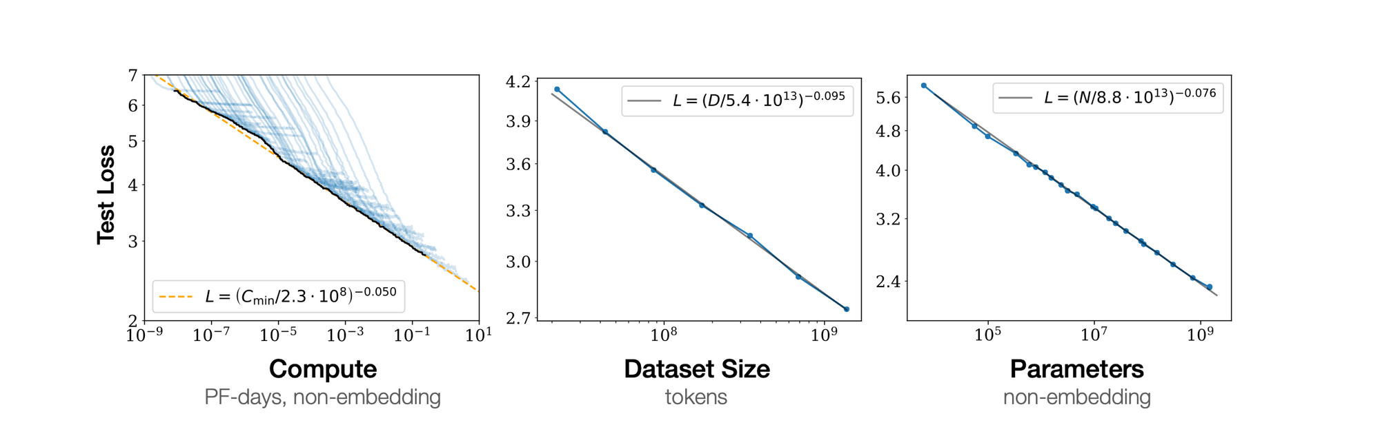
Kaplan et al (OpenAI) deduced that the test loss of a decoder-only Transformer, when trained to autoregressively model language, can be predicted before convergence using a power-law with respect to three pivotal factors: model size (N), dataset size (D), and the amount of training compute (C). In simple english, you can predict your test loss.

Specifically, for models with a limited number of parameters N, trained to convergence on sufficiently large datasets:

$$
L(N) = \left( \frac{N_c}{N} \right)^{\alpha_n}, \quad \alpha_n \approx 0.076, \quad N_c \approx 8.8 \times 10^{13}
$$

And for large models trained with a limited dataset with early stopping:

$$
L(D) = \left( \frac{D_c}{D} \right)^{\alpha_d}, \quad \alpha_d \approx 0.095, \quad D_c \approx 5.4 \times 10^{13}
$$

Given a limited amount of compute, a large dataset, an optimally-sized model, and a fixed batch size:
$$
L(C) = \left( \frac{C_c}{C} \right)^{\alpha_c}, \quad \alpha_c \approx 0.057, \quad C_c \approx 1.6 \times 10^{7}
$$

There is also another formula for optimal use of compute, that is, you define a target loss and end up with the critical value of the compute needed to train with a model of size N and a small batch size B:

$$
L(C_{min}) = \left( \frac{C^{min}_c}{C_{min}} \right)^{{\alpha}^{min}_c}, \quad \alpha^{min}_c \approx 0.050, \quad C^{min}_c \approx 3.5 \times 10^{8}
$$

L signifies the cross-entropy loss and others constans represent coefficients obtained empirically.

Furthermore, a formula for the loss combining N and D was also presented:
$$
L(N, D) = \left( \left( \frac{N_c}{N} \right)^{\frac{\alpha_n}{\alpha_d}} + \frac{D_c}{D} \right)^{\alpha_d}
$$

Conclusions and Implications of the paper:

• Given a fixed computational budget C, the optimal N and D can be determined through constrained optimization.
• Model scale surpasses model shape in significance, specifically for Transformers but probably for other models as well.
• The relationships among N, D, and C are as follows: $$N \propto C^{0.75}, D \propto C^{0.6}$$
• For instance, a 10-fold surge in the computational budget implies the model size should amplify by 5.6, whereas the training tokens should only grow by 3.9 (if the optimal amount of compute is used, you end up with 1.8 tokens).
• The requisite compute to achieve a specified loss for a large model can be approximated.
• Optimal training steps can be chosen to monitor overfitting.
• Larger models will continually exhibit superior performance.

Chinchilla Scaling Law

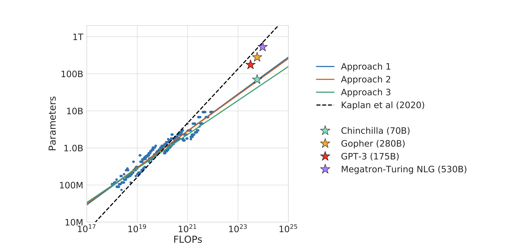
DeepMind proposed a scaling law that closely resembles OpenAI's, albeit with different coefficients. This formulation arose from the risk decomposition, as extensively detailed in the original paper. The coefficients were ascertained by minimizing the Huber loss between the anticipated and observed log loss through the L-BFGS algorithm:

\begin{equation}
L(N,D) = E + \frac{A}{N^\alpha} + \frac{B}{D^\beta}
\end{equation}

The initial term represents the loss for an ideal generative process on the data distribution, ideally corresponding to the entropy of natural text (irreductible loss). The subsequent term emphasizes that a perfectly trained transformer with N parameters does not perform as well as the ideal generative process. The concluding term elucidates the transformer's non-convergent training, resulting from a finite number of optimization steps on a dataset distribution sample.

When optimizing the loss L(N,D) under the constraint C = 6ND , the following optimal allocations for the compute budget concerning model size and data size can be deduced:

\begin{align}
N^* & = G (C/6)^a \\
D^* & = G^{-1} (C/6)^b
\end{align}

where

\begin{align}
b & = \frac{\alpha}{\alpha + \beta} \\
a & = \frac{\beta}{\alpha + \beta} \\
G & = \left(\frac{\alpha A}{\beta B}\right)^{\frac{1}{\alpha + \beta}}.
\end{align}

Where does the C = 6 ND comes from ? The FLOPs required for the forward pass for a single token is approximately 2N (rough estimate - excluding non-embedding parameters - cf https://arxiv.org/pdf/2001.08361.pdf) and 2ND for the entire dataset (one could also give a formula for encoder/decoder separated). The backward pass, due to its nature of computing derivatives for each hidden state and weight (the chain rule), requires about twice as many FLOPs as the forward pass. Therefore, the FLOP count for the backward pass over the entire dataset is approximately 4ND. Summing it up, one complete cycle (forward and backward pass) requires (4+2)ND=6ND FLOPs.

In comparison to OpenAI's scaling law, which promotes a higher budget allocation for model size over data size, the Chinchilla scaling law suggests proportional increases in both sizes, leading to equivalent values for a and b above.