Large Language Models (LLMs) are developed to understand the probability distribution that governs the world language space. Autoregressive models approximate this distribution by predicting subsequent words based on previous context, forming a Markov chain. World knowledge (often referred as parametric knowledge) is stored implicitly within the model's parameters.


Large Language Models (LLMs) are developed to understand the probability distribution that governs the world language space. Autoregressive models approximate this distribution by predicting subsequent words based on previous context, forming a Markov chain. World knowledge (often referred as parametric knowledge) is stored implicitly within the model's parameters.
Earlier language models based on Recurrent Neural Networks (RNNs) or Long Short-Term Memory (LSTM) networks were somewhat effective, yet they had two main drawbacks. First, they struggled with long-term dependencies due to the gradient vanishing/exploding problem. Second, the generation of new tokens was heavily dependent on previous representations, which hindered parallelism in training.
In contrast, LLMs based on the transformer architecture or attention mechanisms can consider distant elements within the input context. Techniques like teacher forcing and masking enabled parallel training.
However, LLMs are typically trained with a limited input context, usually encompassing thousands of tokens. This limitation restricts their practical application in analyzing extensive documents, such as long reports. Various approaches have been proposed to extend the context window of LLMs, which we will explore later.
Despite being trained with massive data and computational resources, LLMs face several challenges. First, they sometimes produce hallucinations or nonsensical responses, albeit plausible. Second, integrating additional, up-to-date knowledge remains a challenge and resource-intensive task, the amount of knowledge a LLM can house is restricted. Addressing these issues could significantly enhance the utility of LLMs, potentially making them a ubiquitous tool in everyday life.
In this post, we will discuss various methods to expand the capabilities of LLMs and make them more efficient. This includes increasing the context length, addressing the issue of hallucinations, and incorporating diverse forms of knowledge.
This post is long, but don't worry , I am providing everything you need to comprehend all the approaches 😉 (at least I tried). I highly recommend that you first read my previous/quick article about GPT in order to start activating your brain 😛.
Good luck 💪!
Before delving deeply into the article, let's first introduce some concepts and studies. I believe this will make understanding later approaches easier. Feel free to skip this section if you are already familiar with the material, or use it as a refresher 😄.
Knowledge distillation (KD) involves training a smaller model, by transferring knowledge from a larger teacher model. In essence, it maps a large and complex network to a simpler one while aiming to maintain good performance. The goal is to retain as much functionality as possible while reducing costs, as the newly learned model carries nearly the same functionality (obtained from the supervision signals during training), albeit with lower accuracy and generalization capability, but more cost-effective in terms of deployment.
KD is closely related to model extraction attacks, where the aim is to learn or steal parameters of a target model, this was highlighted by Xinyi Zhang et al. (2021).
There are several ways to train the student model. Vanilla approaches include simple matching of soft labels such as the teacher model's soft softmax outputs (prediction layer distillation), mimicking the teacher's output distribution difference, attention scores (attention based distillation), or other signals depending on whether you have access to the model or not.
In the context of an LLM, you would want to approximate the policy or distribution of the supervisor model, like GPT4. This can be achieved by reducing the KL divergence between the two distributions.
However, knowledge distillation requires a substantial amount of unsupervised data for training, which can be a challenging requirement to meet. Several techniques have been developed to tackle this issue, such as data augmentation, but there is still room for improvement. There are also other issues to contend with, such as overfitting and generalization.
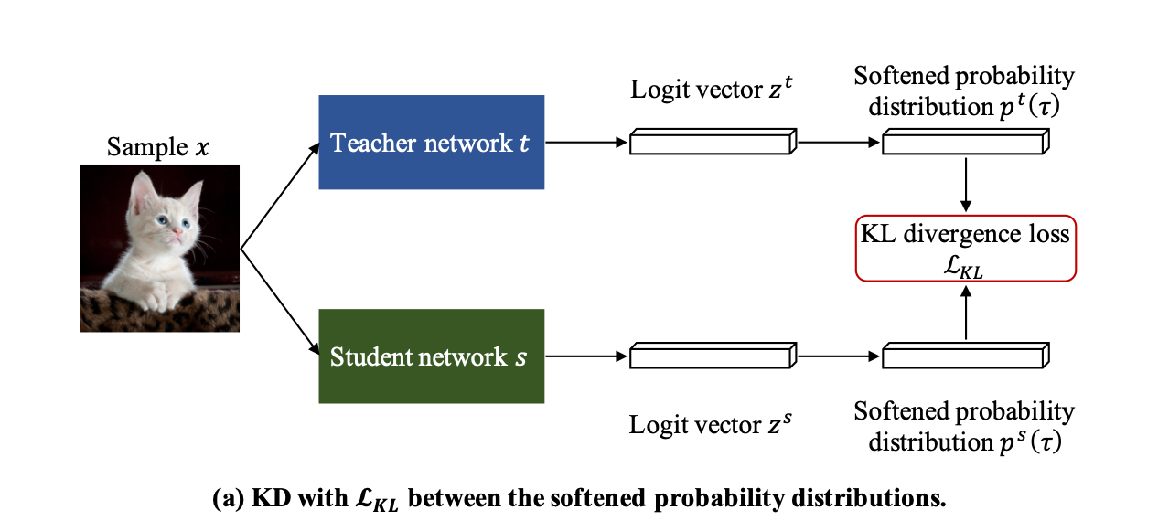
The Kullback-Leibler (KL) divergence loss is a measure of how one probability distribution, \( p \), differs from a reference distribution, \(q\). KL Loss is usually utilized in KD to quantify the divergence between the softened probability distributions of a teacher model and a student model.
Formally, for discrete probability distributions \( P \) and \( Q \) defined on a probability space \( \mathcal{X} \), the KL divergence from \( P \) to \( Q \) is defined as:
$$D_{\text{KL}}(P | Q) = \sum_{x \in \mathcal{X}} P(x) \log \left( \frac{P(x)}{Q(x)} \right)$$
Let's consider a teacher network \( T \) and a student network \( S \). These networks typically produce class probabilities by transforming the logits, computed for each class into a probability using the softmax function. We denote the class probabilities generated by the teacher network \(T \) as \( p^T_i \) and those by the student network \( S \) as \( p^S_i \), respectively. The KD Loss is usually defined as a linear interpolation of traditional cross entropy and KL divergence:
$$L_{\text{KD}} = (1 - \alpha) \left( -\sum_{i=1}^{N} y_i \log(p^S_i(1)) \right) + \alpha \tau^2 \left( \sum_{i=1}^{N} p^T_i(\tau) \log \left( \frac{ p^T_i(\tau)}{p^S_i(\tau)} \right) \right) $$
where \( p^T_i(\tau) = \frac{\exp(t_i/\tau)}{\sum_{j=1}^{K} \exp(t_j/\tau)} \) and \( p^S_i(\tau) = \frac{\exp(s_i/\tau)}{\sum_{j=1}^{K} \exp(s_j/\tau)} \), with \( K \) being the number of classes, \( \tau \) is a temperature scaling hyperparameter, \(y\) is the ground-truth one-hot vector and \(t_i, s_i\) are the the i-th value of the logit vector for the teacher and student network respectively.
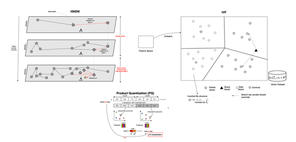
Information Retrieval or IR involves retrieving a collection of relevant documents based on a query. The process begins with indexing a knowledge database, where each document is represented by a unique key. Subsequently, a query calculates the similarity between itself and the various documents in the database. The goal is to identify the top k most similar documents. Techniques for this include projecting documents into an embedding space (continuous) or utilizing sparse representations like TF-IDF. Similarity is then calculated in the resultant vector space, often using cosine similarity.
In this post, particularly in the section on retrieval-augmented models, we will review several papers. Although they have different focuses, their primary motivation is the same: to use augmented knowledge in addition to what is stored implicitly in the model parameters and enhance LLMs efficiency. We refer to this additional knowledge as non-differentiable or non-parametric knowledge.
The goal of indexing is to create a database where each entry is represented by a key. More specifically, the key is a vector that hints at the corresponding value. A traditional approach in IR is to use TF-IDF to create an index with sparse representations. In this representation, each dimension corresponds to a token or term in the selected vocabulary, and the value for each dimension is the occurrence of the term in the document. When we want to retrieve a document, we map it in the vector space (we obtain a sparse vector) and then use the scalar dot product or other similarity measure to retrieve and rank the documents before returning them to the user. There are mainly two problems with this approach.
First, the dimensionality is equal to the number of selected terms, which can quickly become impractical (the curse of dimensionality would render inner product similarity-based search ineffective. ). Second, sparse representations lack context and suffers from vocabulary mismatch. Regardless of how the terms are shuffled, the output of the mapping to our vector space will be the same. In other words, the sparse representation is not dynamic, and each key does not truly represent the contextual data embedded in the corresponding document and does not compress the full context. This is where people started to use learnable, contextualized embeddings, in contrast to Word2Vec, typically using BERT or other transformer-based encoders.
The embedding space obtained using attention-based methods not only reduces the dimension of our input vocabulary space but also ensures that each key (in this case, the encoded document) better represent corresponding document as it embeds the context. Thus, the first and second problems are somewhat solved using contextualized embeddings. Let's now consider two additional problems.
Once you have an embedding that captures important information about a document or passage, you still need to go through all documents, potentially billions, and add to that the fact that they are high-dimensional and need to be ranked and returned. This is not feasible, so people started using a quick approximation to find the most similar documents using the aforementioned embedding space (typically using the dot-product as a similarity score). One of the most known methods is FAISS, a highly efficient similarity search library.
To represent a passage, one can use BERT’s [CLS] token representation, which is assumed to contain enough information (yep, masking is not activated here so the representation can use the full vision of the sequence). The [CLS] embedding of the query is then used to retrieve passages by identifying nearest neighbors using a FAISS index. There are several approaches for sentence embedding and one can also use average pooling over the last hidden layers, we will discuss later some papers that uses this approach later.
Now, we have a contextual, high dimensional (but not excessively high) embedding space to map a corpus of documents and a query for quick similarity search using FAISS or another library.
The last problem is that if our embedding mapping is dynamic, changing during training (suppose you are training the retriever and/or a language model/reader and use the corpus projections for predictions, that is, you do a look up for kNN in that index), our indexing would change as well, and we can't afford to constantly update our index. This is why, as we will discuss in a later section, people tend to update the index after every \(x\) steps, where \(x\) is typically 10 (this is sometimes referred as refreshing strategy, which will update our stale index).
Now, we have a dynamic, learnable embedding space, and we can find the most relevant documents given a query; we'll call that a trainable dense retriever. Once we have the most relevant documents, we can feed them to another model to either extract or generate a synthetic answer; we'll call that a reader. That's enough for now; we will continue our discussion about retrieval-augmented models later.
A latent space is a learnable representation where data inputs are projected in a manner tailored to a specific task. This space typically features reduced dimensions, retaining only the most important features or directions. You can think of it as a form of "learnable" Principal Component Analysis (PCA).
The manifold hypothesis posits that high-dimensional real-world data lies on or near a lower-dimensional manifold. For example, images of a cat, even though they might be represented as high-dimensional vectors (with each pixel as a dimension), likely lie near a lower-dimensional subspace.
Not all dimensions are filled with important or relevant information. Some dimensions might just capture noise or redundant information, and so they might not contribute to the underlying structure of the data (eg. background surfaces). This is why techniques like PCA, GANs, Auto-encoders and VAEs can be effective.
These techniques support the manifold learning concept where they try to learn the underlying geometry or structure (the manifold) of the data. For example, autoencoders can learn to compress data from the input layer into a condensed, or encoded, representation at the hidden layer, and then learn to reconstruct the original data at the output layer. This hidden layer can be thought of as a low-dimensional representation or manifold of the input data (one can think of an Auto-encoder as \(\text{PCA} + \text{PCA}^{-1}\).
Another way to think about the manifold hypothesis is in terms of degrees of freedom. For instance, a human face has a lot of pixels and hence is high-dimensional, but only has a few degrees of freedom (e.g., position of eyes, mouth, nose, etc.). Therefore, we can represent a human face in a lower-dimensional space by capturing these important features.
Yet, manifold hypothesis is still an hypothesis, not a guaranteed property of all datasets. It is also an active area of research to understand when this assumption holds and how to leverage it best for learning algorithms.
Contrastive Learning involves learning a latent space where similar data points are projected close to each other, while dissimilar data points are projected far apart in this space. Formally, the following objective is typically utilized to train an encoder f:
$$L_{\text{CL}} = \mathbb{E}_{(x, x^+) \sim p_{\text{pos}},\; x_i^- \sim p_{\text{data}}} \left[ -\log \frac{e^{f(x^+)^T f(x) / \tau}}{e^{f(x^+)^T f(x) / \tau} + \sum_{i} e^{f(x_i^-)^T f(x) / \tau}} \right]$$
\(x\) and \(x^+\) represent a pair of semantically similar samples from the positive distribution \(p_{\text{pos}}\), forming the positive pair. Conversely, \(x \) and \( x_i^-\) constitute a pair of negative samples, where \( x_i^-\) is randomly drawn from the data distribution \( p_{\text{data}}\) of the independent samples. \(\tau > 0\) is scalar temperature hyperparameter.
Minimizing the aforementioned loss is equivalent to encouraging high similarity scores (dot product between representations) for positive pairs and low scores for negative pairs (as the exponential is always positive), thus enforcing alignment and uniformity of representations.
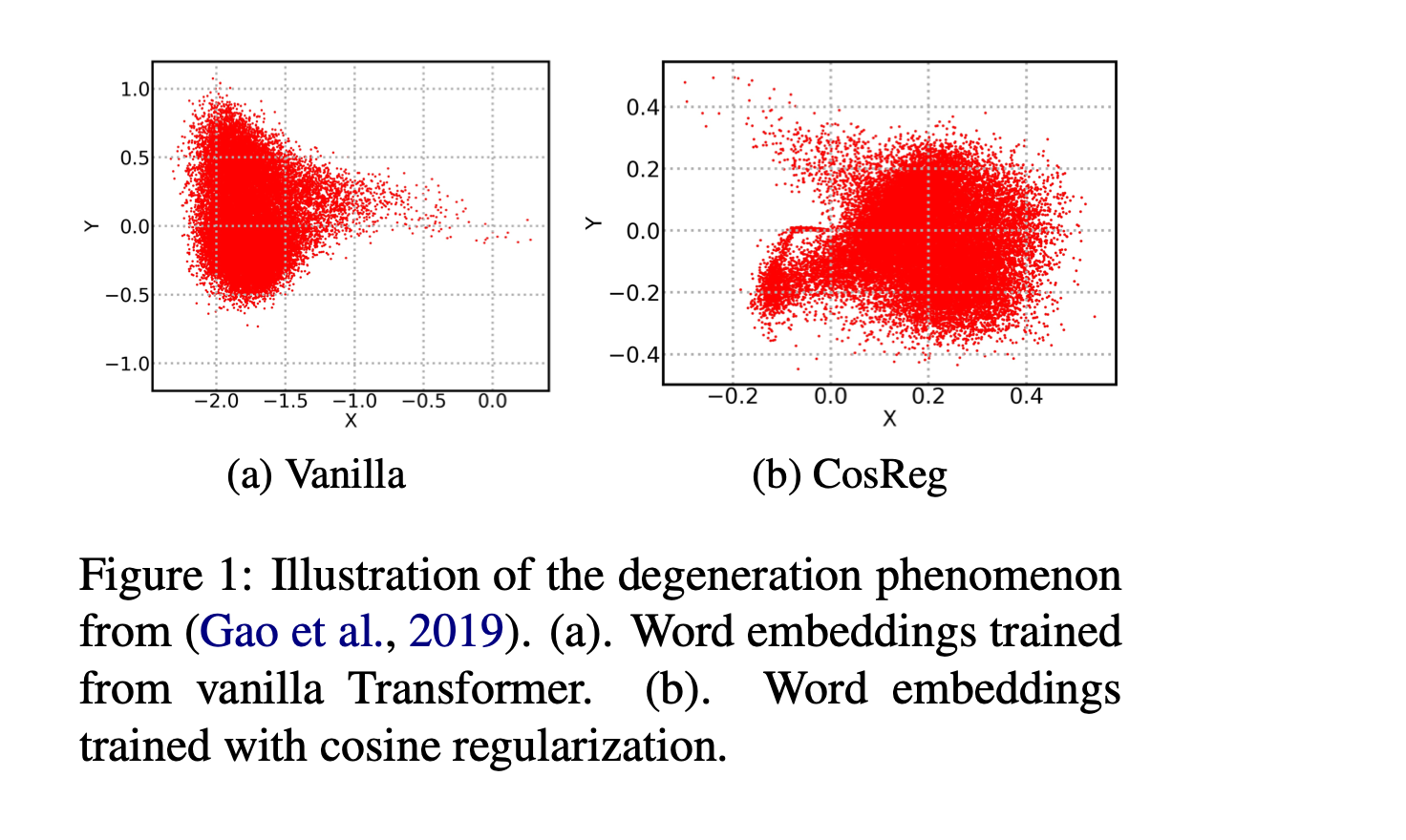
The representation degeneration problem arises because most words in natural language are low-frequency according to Zipf's law.
In such scenarios, when weight tying is used in Transformer based LLMs, the model tends to learn a word embeddings for rare or "non-appeared" tokens that gravitates strongly in the negative direction of other hidden representation of tokens, forming a convex set within a convex cone. You can refer to Jun Gao et al. (2019), who argued that the optimization of rarely appeared word tokens is similar to that of non-appeared word tokens. They explained that the representation degeneration problem stems from the fact that the optimal embedding for rare tokens can be optimized along any uniformly negative direction indefinitely. In simpler terms, this results in an anisotropic distribution of token representations (not evenly distributed across the space they occupy), meaning their representations are confined to a narrow subset of the entire space.
The aforementioned problem curbs the model's semantic expressiveness (as most of those rare words would not be chosen as the inner product is low). Several solutions have been proposed over the years, including contrastive learning, which brings similar sentences closer together in the model and distances dissimilar data points in the representation space. Another solution is to introduce a penalty using Cosine Regularization, which broadens the aperture of the cone, as one can see below.
It should be stressed that the degeneration problem is not limited to static word embeddings, it also extends to contextualized embeddings. Studies [Kawin Ethayarajh et al, Bohan Li et al] have indicated that despite these embeddings being contextual, their latent space often lacks structural features such as isotropy, resulting in incomplete representations. This leads to a scenario where even unrelated words can exhibit overly positive correlations (high scalar product). In simple terms, if your word embedding space is poor, your contextual embeddings will also be affected.
Variational Autoencoders (VAEs) are powerful generative models that creates a lower-dimensional latent representations, from which new data can be sampled. They aim to maximize the Evidence Lower Bound (ELBO) on the data likelihood.
The ELBO of a VAE is given by (the training loss is the negative ELBO):
$$L_{\text{VAE}} = \mathbb{E}_{q_{\phi}(z|x)}[\log p_{\theta}(x|z)] - \text{KL}[q_{\phi}(z|x) || p(z)]$$
Where \(\mathbb{E}\) is the expectation, \(q_{\phi}(z|x)\) is the encoder's distribution, \(p_{\theta}(x|z)\) is the decoder's distribution, KL is the Kullback-Leibler divergence and \(p(z)\) is the prior distribution over the latent variables.
As previously mentioned, representations from common pre-trained language models often suffer from the degeneration problem. One solution is to enforce isotropy in the latent space. In an isotropic latent space, representations of randomly sampled tokens exhibit low cosine similarity and do not cluster in a specific direction.
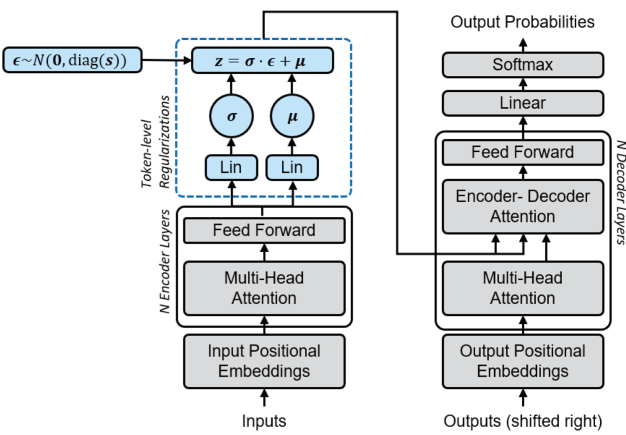
Several studies have proposed using a Gaussian distribution as the latent prior. For instance, the Variational Auto-Transformer (VAT) has demonstrated numerous benefits in regularizing the induced latent representations.
If you are looking for a deep understanding of VAE and other generative models like GANs, you can have a look at Information bottleneck through variational glasses.
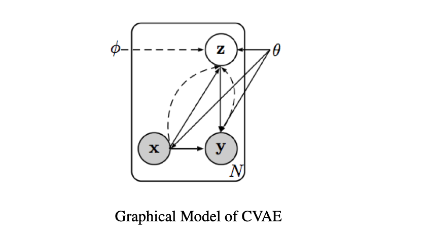
CVAE is an extension of VAE, tailored for supervised learning and conditional generation tasks, offering structured output predictions.
The primary objective of CVAE is to optimize the conditional data log-likelihood, expressed as \(\mathbb{E}_{x,y \sim \mathcal{D}}[\log p_\theta(y|x)] \), which results in the following ELBO:
$$\mathbb{E}_{x,y \sim \mathcal{D}}[\log p_\theta(y|x)] \geq \mathbb{E}_{x,y \sim \mathcal{D}} \left[ \mathbb{E}_{z \sim q_\phi(z|x,y)}[\log p_\theta(y|x, z)] - \mathbb{E}_{x,y \sim \mathcal{D}}[\text{KL}(q_\phi(z|x, y) || p_\theta(z|x))] \right]$$
Here the prior of the latent variable is \(p_\theta(z|x)\). Both prior and posterior networks are trained.
VAEs often suffer from a well-studied phenomenon known as posterior collapse (or KL vanishing), where the posterior distribution of the latent variables becomes identical to the prior distribution, i.e., \( p_{\theta}(z|x) = p(z)\). In other words, the latent variable \(z\) fails to provide meaningful representations.
To address the posterior collapse, various methods have been explored, including the KL thresholding scheme/ Free Bits (FB) [Li et al., Pelsmaeker et al. ]. This approach involves replacing the KL term in the loss function with a hinge loss term that compares each component of the original KL divergence with a constant \( \lambda \), formulated as:
$$L_{\text{KL}} = \sum_{i} \max(\lambda, \text{KL}(q_\phi(z_i | x) || p(z_i)))$$
In statistics, a semiparametric model is a statistical model that combines both parametric and nonparametric components.
LLMs can be augmented with additional non-parametric knowledge sources, which are not stored within the model's parameters but are accessible during runtime through a retrieval module. This approach allows the LLM to dynamically access a broader range of information beyond its trained parameters, enhancing its ability to provide relevant and up-to-date responses, promoting less hallucinations.
Mixture of Experts (MoE) integrates model parallelism, sparsity and ensemble learning, aiming to reduce the memory demands on devices. It involves deploying multiple experts or subnetworks across a range of devices, such as GPUs.
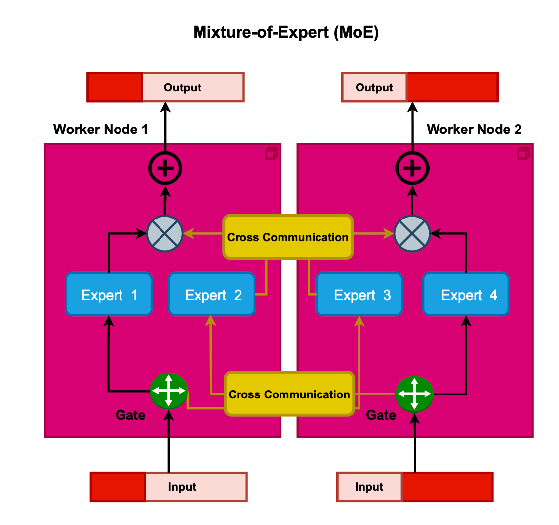
In MoE, tokens are dispatched to a limited set of experts, typically 2, using a trainable routing mechanism. This enables conditional computation at the token level, enhancing model capacity (in other words, only a subset of the model parameters are activated through sparsity). Examples of models that capitalize on the benefits of MoE include GPT-4, Switch Transformers, and GLaM. Additionally, MoE can be applied to the attention layer such as Mixture of Attention Heads. I will not delve deeply into MoE in this post. However, if you are interested in learning more about it and the recent advances in this field, you can refer to my previously published article here.
The self-attention module in Transformers exhibits quadratic complexity with respect to sequence length, which limits its capability and practical utility. Several studies have been undertaken to enhance the efficiency of attention and reduce computational demands. Some of these will be discussed in this section.
As mentioned earlier, training LLMs with extensive sequence lengths is computationally expensive. The Linformer, a variant of the transformer model, addresses this issue by approximating the self-attention mechanism using low-rank matrices.
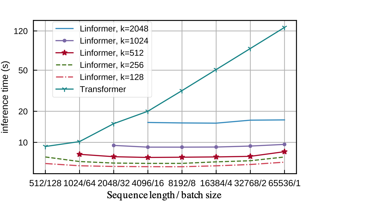
This approximation changes the overall complexity of self-attention from O(n^2) to O(nk), where n is the sequence length, and k is a much smaller dimension representing the low-rank approximation.
This approximation is achieved by adding two linear projection matrices \(E_i\) and \(F_i\) that map the dimensions of the self-attention's keys and values from \(n \times d\) to \(k\times d\), thus significantly reducing the time and space complexity (\(k\) is supposed to be small). The context mapping matrix also goes from \(n \times n\) to \(n\times k\), so at the end you end up with \(n\times d\) matrix housing our contextualised representations.
$$ \text{head}_i = \text{Attention}(QW_i^Q, E_iKW_i^K, F_iVW_i^V) = \text{softmax}\left( \underbrace{\frac{QW_i^Q (E_iKW_i^K)^T}{\sqrt{d_k}}}_{n \times k} \right) \underbrace{F_iVW_i^V}_{k \times d}$$
The Linformer paper also includes a proof, based on the distributional Johnson–Lindenstrauss lemma, demonstrating that for \(k = O(\frac{d}{\epsilon^2})\), one can approximate the contextual embedding of the vanilla self-attention using linear self-attention. You can have a look at the paper for more details (I don't want to overwhelm you with this here).
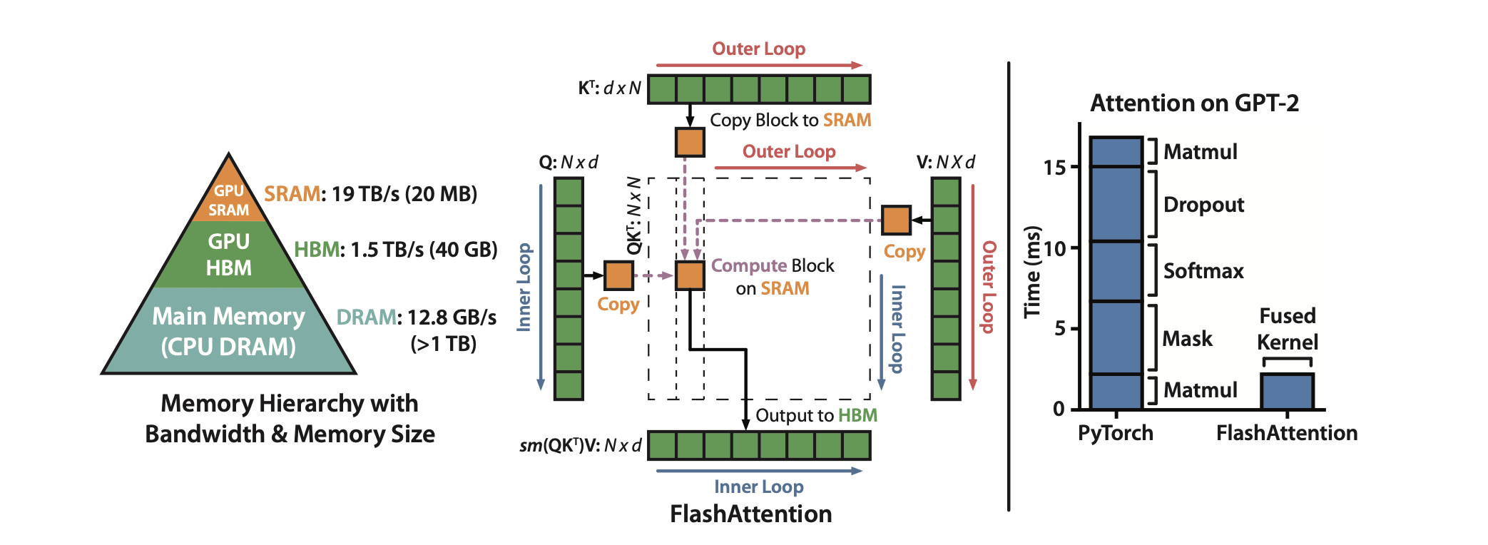
Transformers struggle with long sequences primarily because the standard attention mechanism requires memory accesses that are quadratic in the sequence length. This results in high memory usage and slow processing times.
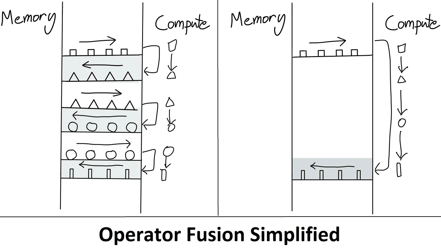
FlashAttention addresses this issue by accessing High Bandwidth Memory (HBM) only once and performing multiple operations consecutively, significantly reducing the number of HBM accesses compared to standard attention mechanisms, enhancing both speed and memory efficiency.
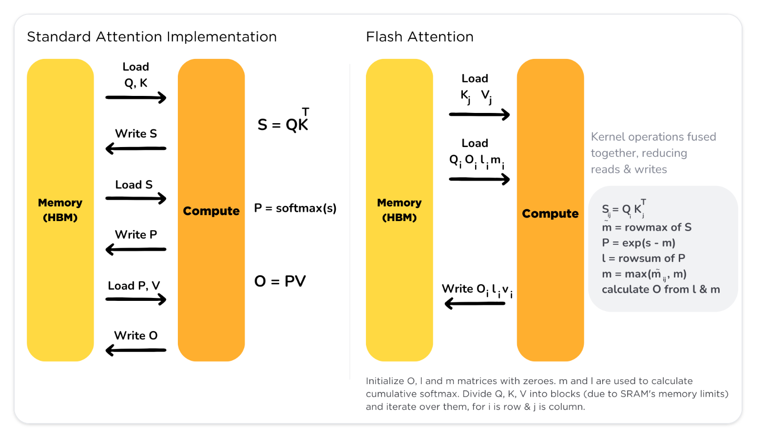
However, a challenge arises as the full attention matrix does not fit in the on-chip SRAM. To overcome this, the paper proposes using tiling and recomputation techniques to avoid the materialization of the large attention matrix.
Basically, it computes self-attention in blocks, involving steps like matrix multiplication, softmax, optional masking and dropout, and another matrix multiplication, all performed after loading the input from HBM and before writing the result back to HBM. This process minimizes the repeated reading and writing of inputs and outputs to and from HBM.
Additionally, the paper introduces an extension of FlashAttention, named Block-Sparse FlashAttention, which approximates attention with an IO complexity lower than FlashAttention, proportional to the sparsity level.
The paper demonstrates that FlashAttention is more efficient than standard attention methods, both in terms of speed and memory usage. It achieves this by fusing all attention operations into a single GPU kernel, reducing the need for multiple memory accesses. In practice, FlashAttention trains Transformers faster than existing methods, achieving a 15% end-to-end wall-clock speedup on BERT-large and a 3× speedup on GPT-2.
Contrary to being an approximation, FlashAttention is an exact computation of attention optimized for fewer HBM accesses, which is a significant bottleneck. The paper suggests that the IO-Aware Deep Learning approach, exemplified by FlashAttention, could be extended beyond attention mechanisms, although this would require substantial engineering efforts.
LLMs are being deployed at an astonishing pace, and finding cost-effective methods to serve them is a hot and active research area. Serving LLMs can be slow and expensive.
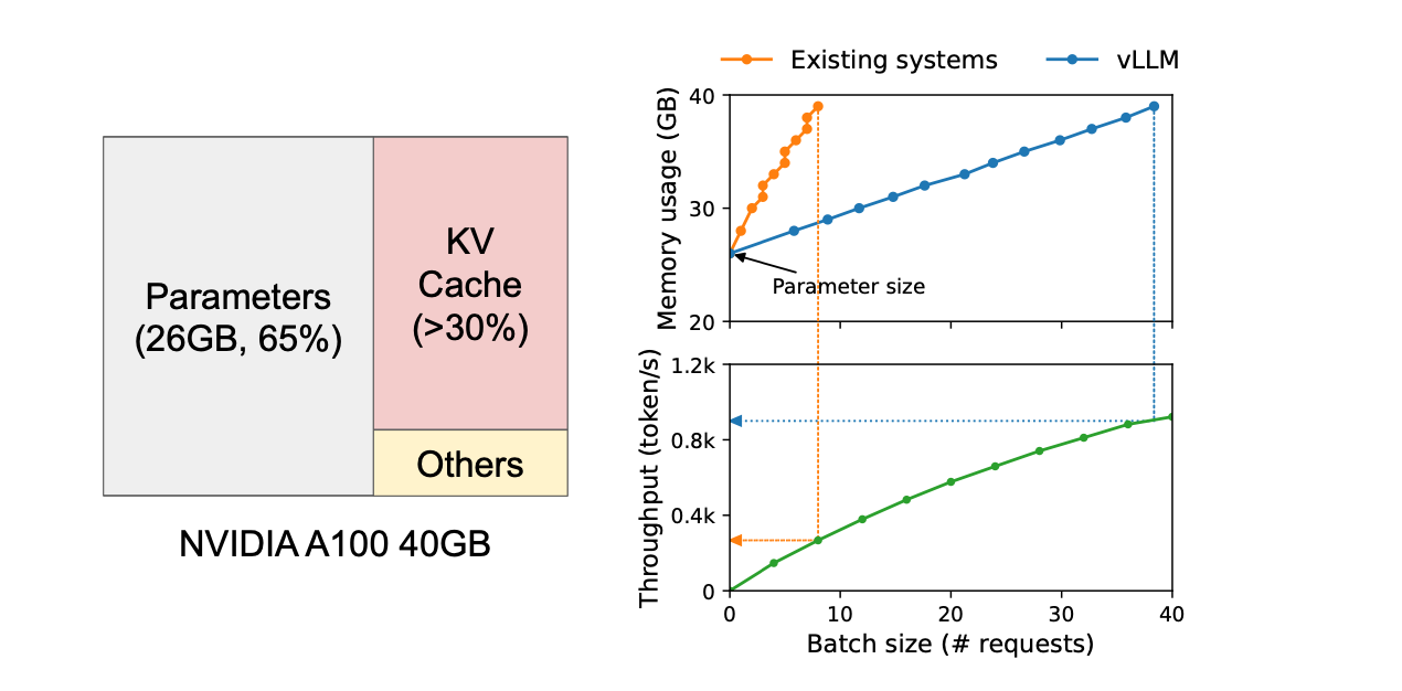
To predict the next token, LLMs must attend to all previous tokens. Typically, previous projections are cached in memory. In the literature, this is often referred to as the KV (Key-Value) Cache. The size of this cache grows as new tokens are predicted and appended, feeding the model until a special token is reached or a specific size limit is met.
Efficient management of this KV cache is crucial, poor management can lead to significant memory waste due to fragmentation, limiting the number of requests and reducing throughput. The PagedAttention/vLLM approach aims to address this issue.
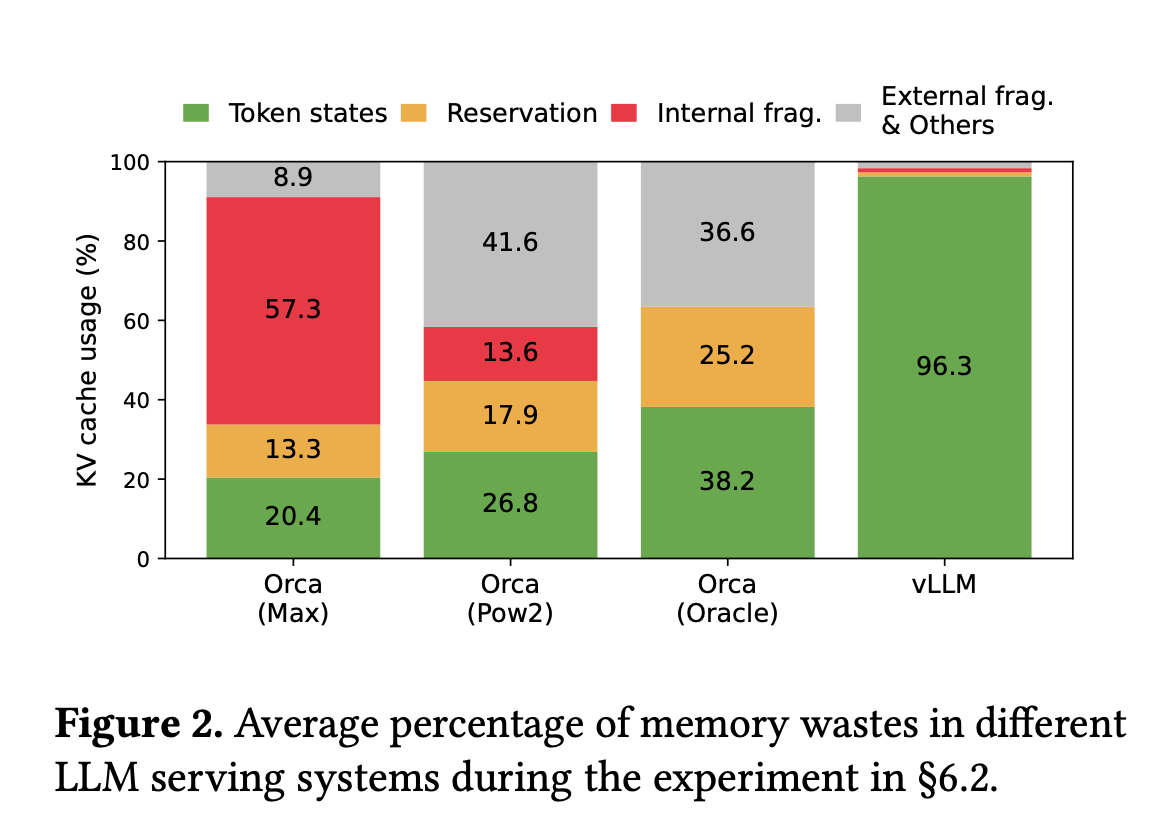
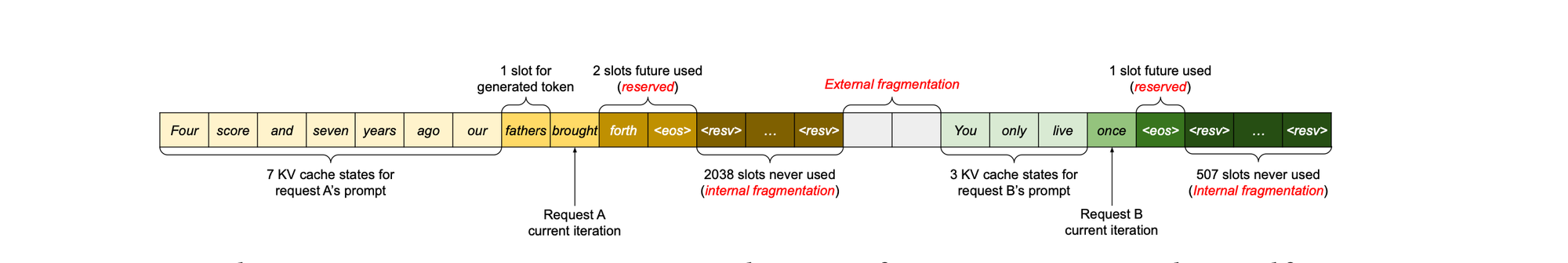
The paper identifies three primary problems with KV cache management: internal fragmentation, due to the unpredictability of the number of tokens a model will generate, reserved memory, which involves pre-allocating memory for future generations that are not used in the current step. and external fragmentation, caused by varying sequence lengths in requests.
Profiling results indicated that only 20.4% to 38.2% of the KV cache memory is utilized for storing actual token states in existing systems.
PagedAttention, inspired by how operating systems manage memory to reduce fragmentation, applies the concepts of virtual memory and paging to KV caching. This approach enables more efficient memory usage for requests.
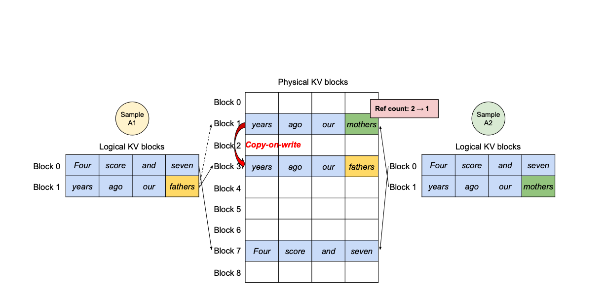
In PagedAttention, the request's KV cache is divided into blocks, each containing a fixed number of tokens' attention keys and values. This method, akin to virtual memory systems in operating systems, allows for blocks to be physically allocated on demand.
PagedAttention achieves zero external fragmentation, while internal fragmentation depends on the block size. This results in a significant improvement in throughput for popular LLMs, with evaluations showing a 2-4 times improvement compared to state-of-the-art systems.
Furthermore, PagedAttention and vLLM enable efficient parallel sampling, where multiple outputs are generated from a single input. This is possible because KV blocks can be shared, enhancing the overall efficiency of LLMs.
While FlashAttention demonstrated significant improvements in memory savings and runtime speedup for Transformers, particularly in handling longer sequence lengths, it did not match the efficiency of optimized matrix-multiply (GEMM) operations (there was still a gap to shrink).
Specifically, FlashAttention achieved only 25-40% of the theoretical maximum FLOPs/s, indicating a need for further optimization.
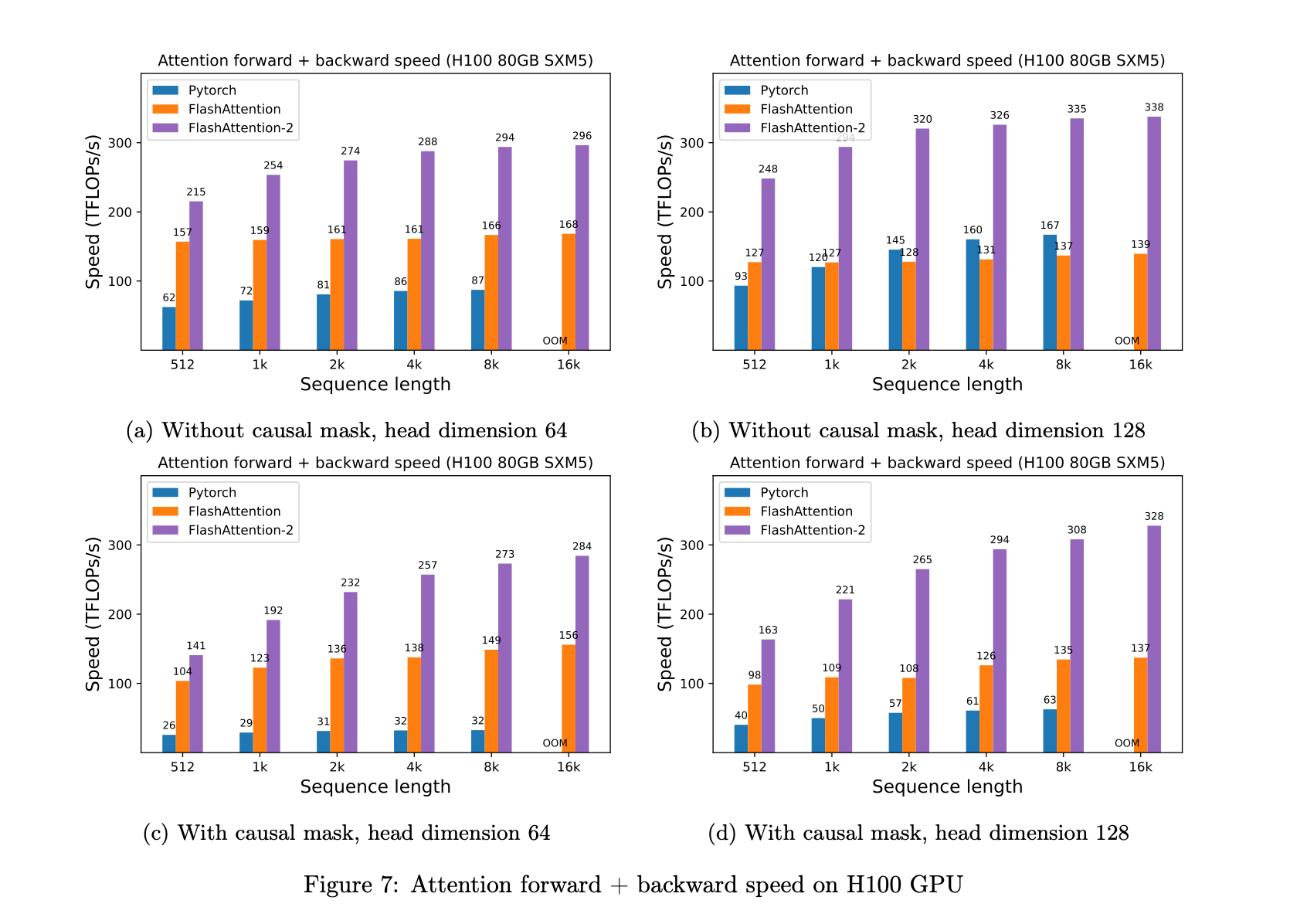
FlashAttention 2 was developed to address these limitations. It introduces better work partitioning and parallelism, specifically targeting the inefficiencies in FlashAttention. The key improvements in FlashAttention 2 include:
These improvements enable FlashAttention 2 to achieve approximately double the speed of FlashAttention, reaching 50-73% of the theoretical maximum FLOPs/s on A100 GPUs.
LongLoRA, an extension of LoRA, is an efficient fine-tuning approach for extending the context window of pre-trained large language models with limited computational cost.
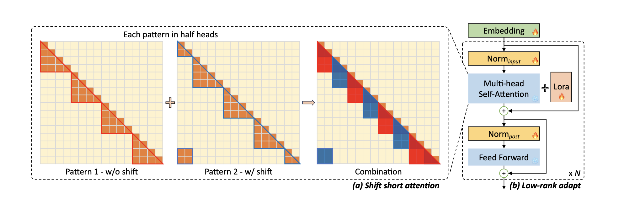
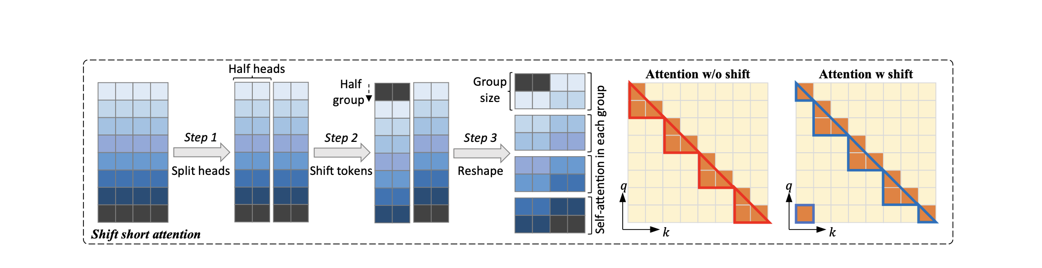
A key innovation is the introduction of Shift Short Attention (S2-Attn), an approximation of vanilla self-attention, which effectively enables context extension while saving significant computational resources.
S2-Attn works by splitting the context length into several groups and conducting self-attention within each group individually. For half of the attention heads, tokens are shifted by half the group size, ensuring that there is an overlap between neighboring groups, this is very important, as it avoid processing groups in isolation, potentially missing out on important context provided by neighboring tokens.
This approach allows for efficient fine-tuning with sparse local attention, while the trained model can retain its original standard self-attention during inference.
Additionally, LongLoRA makes embedding and normalization layers trainable, which is crucial for learning in long contexts, yet these layers constitute only a small proportion of the model's parameters.
The paper demonstrates that LongLoRA achieves comparable performance to full fine-tuning with much lower computational costs.
The performance of Transformer models in various tasks is often limited by their restricted context window, a result of the quadratic complexity arising from the self-attention module. This limitation becomes particularly critical in scenarios where attending to distant tokens is essential, such as in code knowledge bases or tools like GitHub Copilot, and even in audio, and video generation.
The Memorizing Transformer addresses this issue by introducing a memory component that stores previously computed keys and values. This approach allows the model to extend beyond the current window or chunk, providing access to a broader, more relevant context. This is crucial because the core idea of attention is to selectively focus on relevant information. Not all previous tokens are pertinent, and it's inefficient to compute attention scores for all of them, especially when computational resources and time are limited.
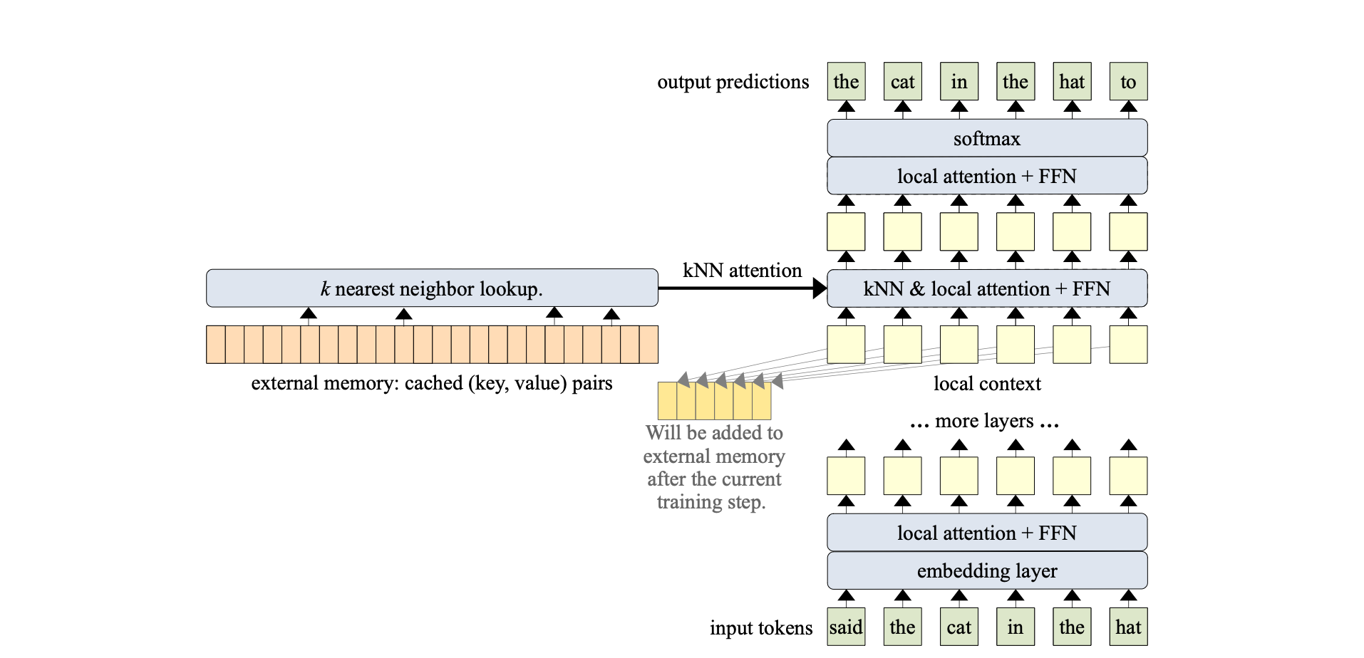
Specifically, the Memorizing Transformer introduces a kNN (k-Nearest Neighbors) augmented attention layer. This layer functions by storing all previous key-value pairs in an external non-differentiable memory. This setup enables the model to access a broader range of contextual information, allowing it to selectively attend to the most relevant information from this external memory.
More specifically, A 12-layer, decoder-only Transformer was utilized. The memory mechanism was applied exclusively to a single layer; more precisely, k = 32 was employed. Furthermore, the 9th layer was designated as the kNN-augmented attention layer.
The Memorizing Transformer calculates contextual projections for each token in two distinct ways:
After computing these two sets of hidden states or representations, the Memorizing Transformer integrates them using a learned gating mechanism. This mechanism involves a bias term that is learned for each attention head. Therefore, if the model has 10 attention heads, there will be 10 distinct gates.
Each gate effectively combines the results from attending to the external memory with those from attending to the local context. This integration produces the final output of the kNN-augmented attention layer as follows:
$$ g = \sigma(b_g), \quad V_a = V_m \odot g + V_c \odot (1 - g)$$
Where \(V_m \) is the outcome of attending to external memory, and \(V_c \) is the result of attending to the local context, \(b_g\) is the learned per-head bias and \(V_a \) is the combined result.
This approach enables the Memorizing Transformer to effectively manage larger contexts, thereby significantly improving its performance on tasks that require an understanding of long-term dependencies and extensive context awareness.
Unlimiformer is similar to Memory Transformers. It augments existing pretrained encoder-decoder transformers to manage inputs of unlimited length. This enhancement is realized by delegating the cross-attention computation to a singular kNN index.
In this approach, each attention head within every decoder layer retrieves its top-k keys from this index, thereby avoiding the need to attend to every key in the input. In essence, it circumvents processing all of the encoder’s top-layer hidden states.
For lengthy inputs exceeding the model's context window capacity, the data is segmented and fed to the encoder in chunks. Subsequently, only the central half of the encoded vectors from each segment is retained. This strategy ensures that the encodings possess adequate context on both sides. Furthermore, the encoded inputs are indexed in a kNN index, utilizing a library such as FAISS for efficient similarity search.
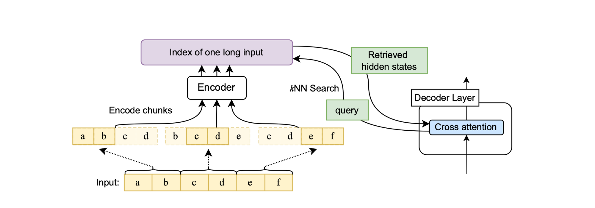
There are primarily two differences between Memorizing Transformers and Unlimiformer. Firstly, Memorizing Transformers are decoder-only transformers, whereas Unlimiformer is based on an encoder-decoder architecture. Additionally, while both Unlimiformer and Memorizing Transformers cache past input keys/values to extend the context window, Memorizing Transformers adopt a more straightforward approach. Consider \( h_d \) as the decoder hidden state and \( h_e \) as the encoder's last layer hidden state. The standard cross-attention computation for a single head in a transformer is given by:
\begin{equation}
\text{Attn}(Q, K, V) = \text{softmax}\left(\frac{QK^T}{\sqrt{d_k}}\right)
\end{equation}
where \( Q = h_d W_q \) is the product of the decoder states \( h_d \) and the query weight matrix \( W_q \); the keys \( K = h_e W_k \) are the product of the last encoder hidden states \( h_e \) with the key weight matrix \( W_k \); and \( V = h_e W_v \) is similarly the product of \( h_e \) with the value weight matrix \( W_v \).
The goal is to retrieve a set of keys \( K_{\text{best}} \) that maximize \( QK^T \), with the size of \( K_{\text{best}} \) fixed to the size of the model’s optimal context window. \( W_q \), \( W_k \), and \( W_v \) are layer-specific and head-specific. Thus, naively creating an index from the keys \( K = h_e W_k \) and querying this index using the query vectors will require constructing separate indexes for the keys and values at each layer and each head, for a total of \( 2 \times L \times H \) indexes, where \( L \) is the number of decoder layers and \( H \) is the number of attention heads. Creating a separate index for each attention head in each decoder layer is both time-intensive and space-intensive.
Unlimiformer, on the other hand, uses a single index across all attention heads and all decoder layers. They leverage the fact that the dot-product part of the transformer’s attention computation can be rewritten as:
\begin{equation}
QK^T = (h_d W_q)(h_e W_k)^T = (h_d W_q) W_k^T h_e^T = h_d W_q W_k^T h_e^T
\end{equation}
Thus, the retrieval step can be formulated as electing the encoder hidden states \( h_e \) that maximize \( h_d W_q W_k^T h_e^T \). This rewriting has two major advantages: first, there is no need to index the keys for each head and layer separately, one can create a single index of the hidden states \( h_e \) only, and just project the queries to \( h_d W_q W_k^T \) using head-specific and layer-specific \( W_q \) and \( W_k \), second, the values can be calculated trivially given \( h_e \), so there is no need to store the values in a separate index from the keys before decoding. Thus, instead of constructing \( 2 \times L \times H \) indexes and retrieving from all indexes during each decoding step, Unlimiformer construct a single index from \( h_e \) and retrieve from it by just projecting the decoder hidden states to per-head per-layer \( h_d W_q W_k^T \). Since indexes can be offloaded to the CPU memory, Unlimiformer’s input length is practically unlimited.
Unlike some other models that add trainable attention gates (e.g. Memorizing Transformers), Unlimiformer is non-parametric and does not introduce additional parameters. This makes it more efficient and easier to integrate with existing models.
Additionally, Unlimiformer process even 500k token-long inputs from the BookSum dataset, without any input truncation at test time and without additional learned weights and without modifying the definition of the mathematical definition of the transformer’s standard dot-product attention.
One of the challenges with traditional transformer models is their limitation to a fixed context length. This often necessitates fragmenting corpora inputs into segments of manageable size for training, leading to a loss of context across these fragments.
While transformers represent an improvement over traditional RNN or LSTM models in handling long-term dependencies, they do not completely solve this issue. A novel approach to address this is by integrating concepts from RNNs into deep self-attention networks, leading to the development of Transformer XL.
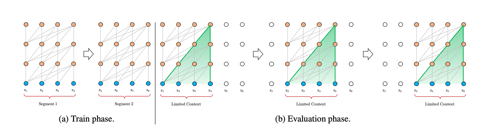
Transformer XL integrates attention mechanisms with recurrence, creating a synergy that effectively addresses the limitations of both RNNs and attention-based models like the standard Transformer.
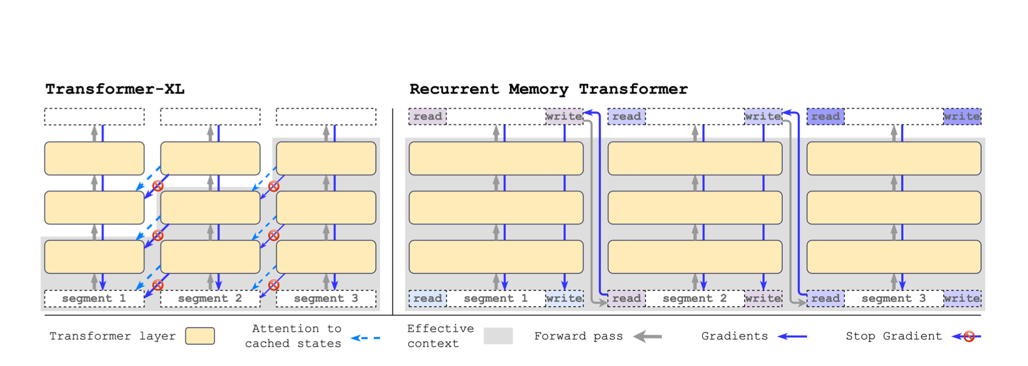
Unlike traditional models, Transformer XL's training process doesn't limit itself to the current segment of data. Instead, it incorporates information from previous segments during the forward pass. This is achieved by caching and reusing previous hidden states, which serve as an extended context for the model. This extended context allows the model to attend to a much larger span of information, limited only by the capacity of the GPU memory.
However, it's important to note that these reused hidden states are not updated during the optimization of subsequent segments. They are concatenated to the current hidden states, providing a continuous and extended context. This approach allows Transformer XL to effectively capture long-term dependencies, overcoming the context fragmentation issue that plagues fixed-length context models.
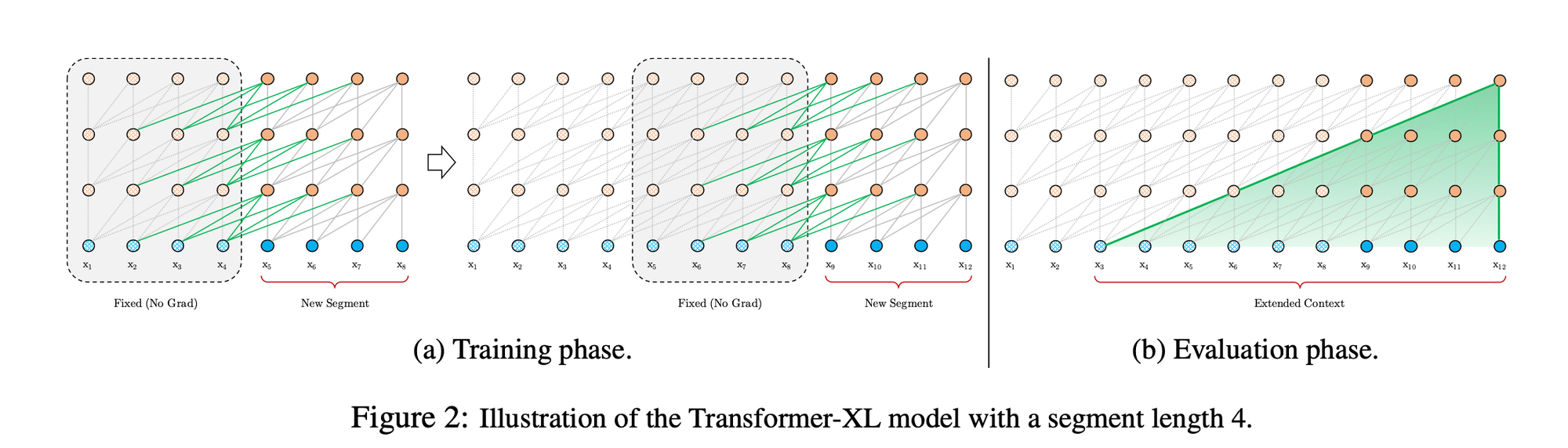
Formally, denoting the n-th layer hidden state sequence produced for the \(\tau\)-th segment \(s_{\tau}\) by \(h_{n}^{\tau} \in \mathbb{R}^{L \times d}\), where \(d\) is the hidden dimension. Then, the n-th layer hidden state for segment \(s_{\tau+1}\) is produced as follows:
$$\begin{align*} \hat{h}_{n-1}^{\tau + 1} &= \text{SG}(h_{n-1}^{\tau}) \circ h_{n-1}^{\tau+1}, \\ q_{n}^{\tau+1}, k_{n}^{\tau+1}, v_{n}^{\tau+1} &= h_{n-1}^{\tau+1}W_{q}^{\top}, \hat{h}_{n-1}^{\tau+1}W_{k}^{\top}, \hat{h}_{n-1}^{\tau+1}W_{v}^{\top}, \\ h_{n}^{\tau+1} &= \text{Transformer-Layer}(q_{n}^{\tau+1}, k_{n}^{\tau+1}, v_{n}^{\tau+1}). \end{align*}$$
Where the function \(\text{SG}(\cdot)\) stands for stop-gradient (in other words , we detach the memory tensors from the AD graph), the notation \(\circ\) indicates the concatenation of two hidden sequences along the length dimension, and \(W_{k,q,v}\) the projection matrices. Compared to the vanilla Transformer, the difference lies in that the key \(k_{n}^{\tau+1}\) and value \(v_{n}^{\tau+1}\) are conditioned on the extended context \(h_{n-1}^{\tau}\) cached from the previous segment.
A critical aspect of extending the context in Transformer XL is the management of positional encoding self-attention layers. This is essential because the model aims to reuse previous hidden states, and naive approaches could negatively affect performance. Positional encoding is vital as it informs the model about the sequence order for effective attention mechanisms. The paper introduces the concept of relative positional encodings, which will be discussed later, as opposed to absolute ones.
The Recurrent Memory Transformer (RMT) is a novel architecture that enhances the Transformer model by incorporating a memory mechanism. This mechanism is implemented through special memory tokens added to the input sequence, allowing the model to store and process both local and global context effectively. These memory tokens enable the passage of information between segments of a long sequence, making the model recurrent and removing limitations on input sequence length.
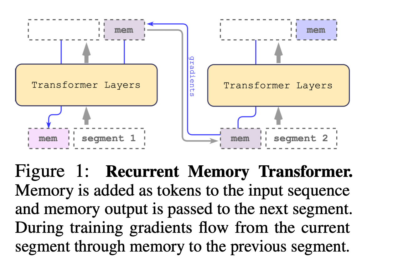
In RMT, memory tokens are added at both the beginning and the end of the segment tokens representations. The initial group of memory tokens acts as a read memory, enabling sequence tokens to attend to memory states produced in the previous segment. The final group serves as a write memory, updating representations stored in the memory based on the current segment tokens (what is interesting to note is that those tokens have access to all the segment though attention). This design allows for efficient information flow and memory updating across segments.
$$ \tilde{H}^0_{\tau} = [H^{\text{mem}}_{\tau} \circ H^0_{\tau} \circ H^{\text{mem}}_{\tau}],$$
$$ \bar{H}^N_{\tau} = \text{Transformer}(\tilde{H}^0_{\tau}),$$
$$[H^{\text{read}}_{\tau} \circ H^N_{\tau} \circ H^{\text{write}}_{\tau}] := \bar{H}^N_{\tau}$$
$$ H^{\text{mem}}_{\tau + 1} = H^{\text{write}}_{\tau},$$
$$ \tilde{H}^0_{\tau + 1} = [H^{\text{mem}}_{\tau+1} \circ H^0_{\tau+1} \circ H^{\text{mem}}_{\tau+1}],$$
RMT differs from Transformer-XL in its handling of memory. Unlike Transformer-XL, where memory gradients flow are stopped between segments, RMT uses Backpropagation Through Time (BPTT) to propagate gradients to previous segments, enhancing its ability to learn from longer sequences. Additionally, with RMT, you only need to stores \(m\) memory vectors per segment while the Transformer-XL needs \(m \times N\) vectors (N here is the number of layers, so RMT is not layer specific and the same m tokens are added at the beginning and end of the sequence).
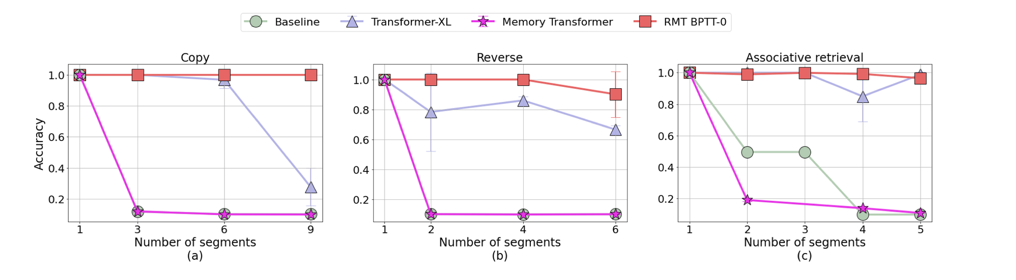
The experiments conducted with RMT demonstrate its effectiveness in tasks requiring the preservation of long-term dependencies across multiple input segments. Additionally, RMT matches the performance of Transformer-XL in language modeling when using smaller memory sizes and surpasses it in tasks demanding the processing of longer sequences.
One line of research enhancing LLMs efficiency involves Retrieval-based LLMs. The concept is as follows: suppose you have a query or question, and your pretrained LLM lacks knowledge in this new area, or the model may not be sufficiently trained on the specific data distribution in question, such as a rare or tail distribution scenario. To address this, a static (potentially non-static) knowledge corpora is employed (non-parametric knowledge). The query retrieves relevant documents from this corpus, and this additional related context is then aggregated with the input to assist the LLM in better understanding the task at hand, potentially reducing the likelihood of hallucinations. Retrieved documents are necessarily concatenated with the input query, passages could also be feed in term of distribution, in other words, the aggregation could be implicit or explicit.
Specifically, Retrieval-Augmented Paradigm can be formulated as follows: in standard text generation, the process involves an input \( x \) and an output \( y \), where \( y = a_{\theta}(x) \). Retrieval-augmented LLMs introduce an additional, relevant context \( z \), so the output becomes \( y = a_{\theta}(x, z) \). In this model, the answer depends both on the input \( x \) and the context \( z \), which resides in training corpora or external datasets. This approach specifically involves using a retriever \( R \) that knows how to find relevant documents from the corpus \( Z \), that is, \( p_{\phi}(z|x) \), (basically it learns how to score), and a decoder or generator \( D \) that generates the response \( q_{\theta}(y|z, x) \). The retriever \( R \) selects the pertinent context from the knowledge source using specific metrics for similarity calculation, such as cosine similarity, after mapping the query and documents to a low-dimensional latent sparse. The mapping could also be done using sparse vector retrieval like TF-IDF which utilizes inverted index matching (so you have choice between embedding and term based similarity). This paradigm can also be expressed in probabilistic terms:
$$p(y|x) = \sum_{z \in \text{top-k (Z)}} p(y|x, z)p(z|x)$$
In the above formula, we select the top-k most relevant passages as it is usually infeasible to go through all the outsourced corpora \(Z\).
To further elucidate the retrieval-augmented paradigm, we will look later at some papers.
The objective of question answering systems is to autonomously provide answers to queries posed in natural language by humans. Open-domain question answering (ODQA) has garnered significant attention recently.
Basically, ODQA refers to the task of deriving answers from an extensive collection of documents. In ODQA, the system identifies one or a set of relevant documents from a large corpora and then processes the result to ascertain the most pertinent answer to the posed question.
A prevalent methodology in ODQA tasks is the two-stage retriever-reader framework. In this framework, a retriever initially selects relevant candidate passages, followed by a reader that extracts the answers from these passages. An alternative approach is the retriever-generator framework, where the generator produces synthetic responses, as opposed to locating the answer within the selected and retrieved document(s).
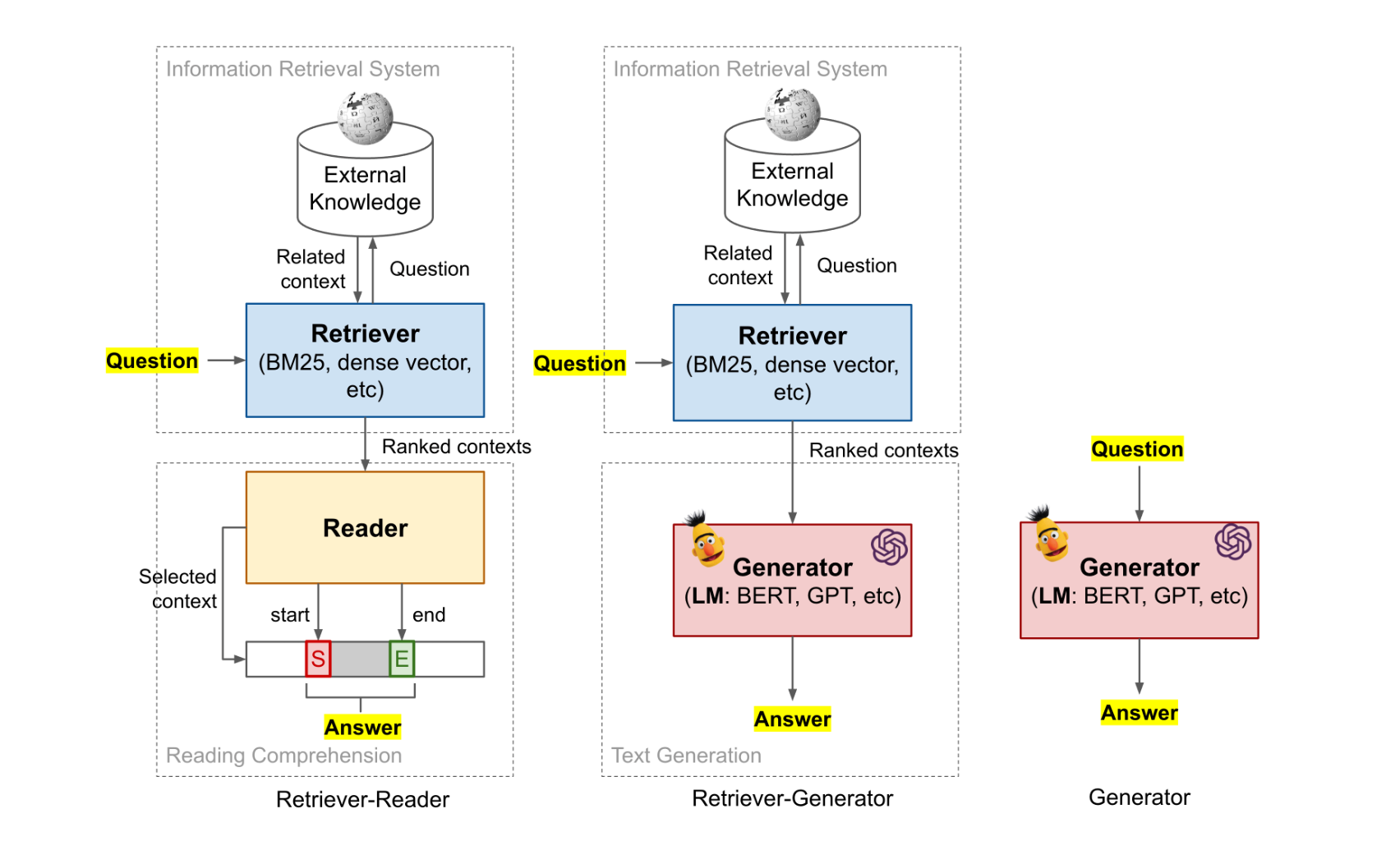
The Retriever-Reader framework, as its name suggests, consists of two main components: the Retriever and the Reader.
The Retriever functions analogously to Information Retrieval (IR) systems and encompasses modules like Deep Neural Networks (DNNs), which helps, through their learnable latent space, in identifying pertinent documents for a specific query.
On the other hand, the Reader, generally realized through a DNN (e.g. BERT), is tasked with extracting answers from the chosen documents. Typically predicting the start and end tokens of the answer within a gold passage (this assumes that the answer consists of a contiguous sequence of tokens that can be found in attend document \(z\), similar to open-book exam).
The framework's Retriever is further categorized into Sparse Retriever and Dense Retriever. The Sparse Retriever employs sparse representations like TF-IDF, whereas the Dense Retriever utilizes dense latent representations of queries and passages or documents.
Just so that you are not confused later, a typical retriever consists of an encoder (which can be either frozen or trainable, commonly based on BERT) and a dot product similarity search engine. The retriever compares the embedding of a query with the embeddings of all indexed passages, using high efficient library like FAISS. The receiver then delegates the top k most similar passages to the reader, which infers the answer from these passages.
Additionally, both the retriever and the reader can be frozen, leveraging the emergent ability of LLMs.
When you read about training the receiver, it refers to training the differentiable parametric module of the retriever, which is typically the encoder. The training tunes the projection to better approximate relevance for answering questions.
Several recent techniques, such as distillation, have been used to supervise the retriever projection more effectively, resulting in better representation in the latent space with improved context alignment. We will discuss this further later.
The Retriever-Generator framework approach aims to marry both generative modeling and retrieval methodologies. Compared to the retriever-reader approach, the retriever-generator also features staged components. The first stage is a retrieval module, similar to that in the retriever-reader framework. However, the second stage employs generative models. The generator G, often a transformer-based architecture, such as GPT2, takes the input sequence x and the retrieved documents, and generates an answer token by token, rather than extracting it or identifying start/end positions of the answer in the retrieved document.
Before going through some papers, let's summarize: the retriever module includes an encoder that creates a vector space from a large corpus. The basis of this vector space can either be trained, as in the case of ATLAS, or remain fixed, as in RETRO. Subsequently, a vector index is created using a highly efficient library for vector retrieval, such as FAISS. Given a query, the encoder projects it into the vector space (the encoder could be the same or different from the one used for the indexed documents) and then outputs the top-k similar results. Some studies propose training the retriever in conjunction with another language model, like GPT-2, while others use a fixed, unmodifiable retriever/decoder. For example, ATLAS, which we will discuss later, trains both the retriever and the language model in an end-to-end manner. This approach is specifically designed to leverage feedback signals from the language model to enhance the encoding capabilities of the retriever.
REALM enhances a model's capability by enabling it to access external knowledge sources like Wikipedia, moving beyond relying solely on internal knowledge stored within the model's parameters for inference.
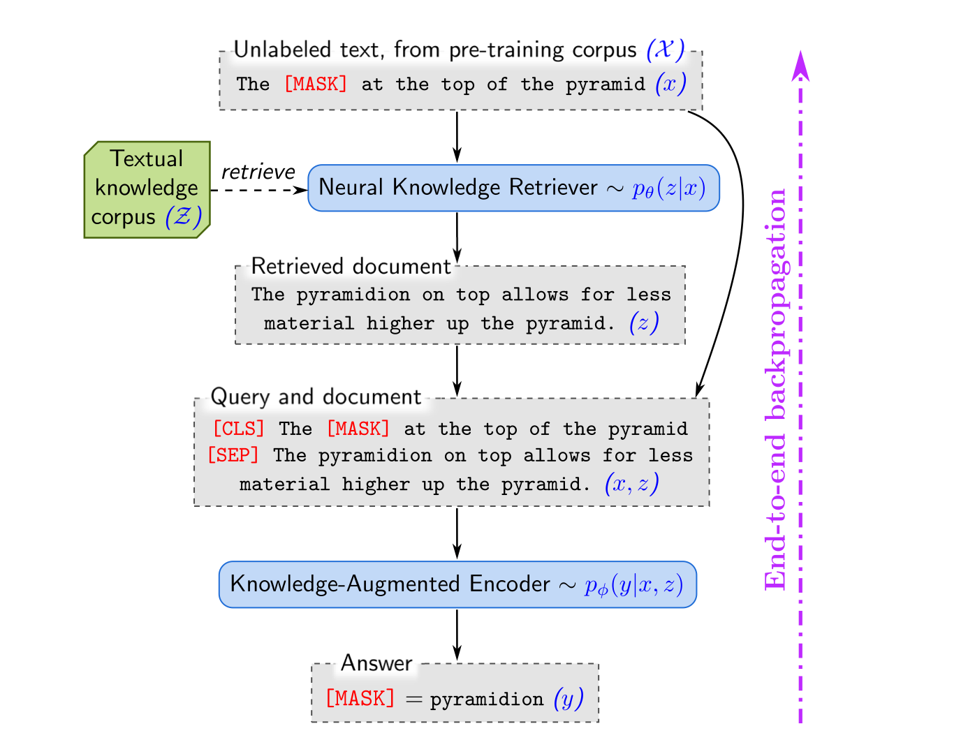
REALM introduces a trainable retrieval module, basically an encoder, designed to identify query-relevant documents from an external index. This approach enriches the model's responses to queries by utilizing both the question and retrieved related context.
One of the challenges in integrating a retriever is the impracticality of processing millions of candidate documents from the external corpus in each pre-training step. To address this, REALM employs Maximum Inner Product Search (MIPS) algorithms to efficiently find the top k documents. However, since MIPS relies on pre-computed embeddings, it is not feasible to recompute embeddings for all documents at every step. To manage this, REALM uses a 'refresh' strategy to deal with stale indexing (where basically the basis of the vector space used for the projection has changed during training). Every few hundred steps, a re-embedding and re-indexing of all documents is performed. This approach balances the need for up-to-date embeddings with the practical constraints of large-scale document processing.
In the retrieval module of REALM, embedding functions, typically based on BERT-style Transformers, are used to generate representations of input sequences and documents from an external corpora. These embeddings are then projected to a lower dimensional space using trainable projections, facilitating the comparison and retrieval process.
To estimate the probability of a document given an input, that is \(p(z|x)\), REALM employs a dense inner product followed by a softmax distribution. This approach allows the model to efficiently retrieve the most relevant documents from a large corpus based on the input query.
In the prediction phase, REALM combines the input \(x\) and the retrieved document \(z\) into a unified sequence. This combined sequence is then processed by a distinct Transformer model, separate from the one used in the retrieval process. This setup facilitates comprehensive cross-attention between the input and the retrieved document before making the final prediction for the output y. Both the knowledge-augmented encoder, which processes this combined sequence, and the knowledge retriever are designed as differentiable neural networks, allowing for end-to-end training and optimization.
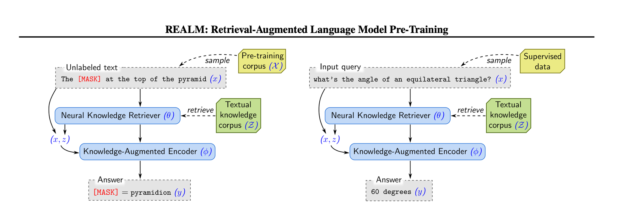
As shown above, REALM undergoes unsupervised pre-training with masked salient spans, followed by fine-tuning using task QA data of interest.
REALM demonstrates significant improvements in accuracy by augmenting its responses with retrieved passages. In Open-QA benchmarks, it outperforms previous methods by a considerable margin, achieving 4-16% absolute accuracy improvements.
Recently, continuous latent representations of word embeddings have emerged as a promising solution for information retrieval. This approach contrasts with traditional, sparse bag-of-words representations such as TF-IDF or BM25. The Dense Passage Retriever (DPR) was proposed for end-to-end open-domain question answering.
Fundamentally, DPR comprises a Retriever and a Reader. The Retriever, for each query \(q\), returns a list of the \(k\) most relevant documents from a given corpus, such as Wikipedia. These results, along with the original query, are then fed to the Reader. The Reader utilizes this additional non-parametric context to answer the query (by predicting the start and end tokens).
DPR encodes the query and documents using two corresponding BERT-based encoders to obtain d-dimensional real-valued vectors. These dense representation vectors are then used to compute relevance scores using a dot product, which is highly correlated with cosine similarity and L2 distance. The top k retrieval problem is thus recast as a nearest neighbor search in vector space, performed efficiently with a k-nearest neighbors library like FAISS.
The document encoder builds an index for all M passages used for retrieval. Both encoders (document and query) are trained in such a way that the dot product yields a relevant similarity score between the document and the query. In other words, a relevant query-document pair should have a high similarity score, while dissimilar pairs should have a low score. The paper used kind of contrastive loss, as shown below:
$$L(q_i, p^+_i, p^-_{i,1}, \ldots, p^-_{i,n}) = -\log \frac{e^{\text{sim}(q_i, p^+_i)}}{e^{\text{sim}(q_i, p^+_i)} + \sum_{j=1}^{n} e^{\text{sim}(q_i, p^-_{i,j})}}$$
The reader component in DPR utilizes BERT-base and processes each candidate context concatenated with the question q. Essentially, the reader predicts the start and end tokens of the answer. This involves a linear layer applied on top of BERT, which predicts the start and end logits for each token based on the final hidden layer representations.
For each retrieved document, the reader assigns a passage selection score. It also extracts an answer span from each passage and assigns a span score. The final answer is determined as the best span from the passage with the highest passage selection score. The reader employs the learned representation of the [CLS] token to predict the overall relevance of the context to the question (the contextual projection of [CLS] token is commonly used as a sentence representation) .
Formally, the probabilities of a token being the start/end positions of an answer span and a passage being selected are defined as:
$$ \begin{align*} P_{\text{start}, i}(s) &= \text{softmax}(P_i \cdot w_{\text{start}})_{s} \\ P_{\text{end}, i}(t) &= \text{softmax}(P_i \cdot w_{\text{end}})_{t} \\ P_{\text{selected}}(i) &= \text{softmax}(\hat{P}^{t} \cdot w_{\text{selected}})_{i} \end{align*} $$
Where \(P_i\) is the representation for the i-th passage (a matrix), and \(\hat{P}\) is the matrix where each column corresponds to the the learned representation of [CLS], that is, the contextual representation of each passage.
The span score from the s-th to t-th words in the i-th passage is defined as:
$$\text{Span score} = P_{\text{start}, i}(s) \times P_{\text{end}, i}(t)$$
To facilitate rapid retrieval from a vast collection of documents, DPR incorporates FAISS, an efficient library capable of performing similarity searches and clustering dense vectors. This enables the construction of a high-speed inverted index.
In term of results, across a broad spectrum of open-domain QA datasets, the dense retriever significantly outperforms a robust Lucene-BM25 system, showing an absolute improvement of 9%-19% in top-20 passage retrieval accuracy. This enhancement contributes to our end-to-end QA system setting new benchmarks in multiple open-domain QA challenges.
Overall, the retriever's objective is to minimize the number of candidate passages that the reader must evaluate. As we will discuss later, DPR can be integrated with a general model like GPT2, T5 or BART for synthetic answer generation.
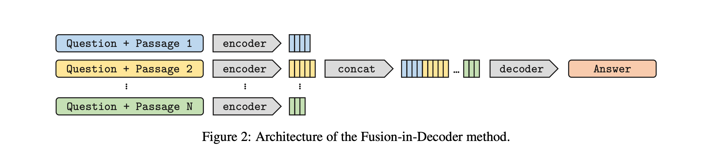
The Fusion Encoder-Decoder (FiD) leverages the strengths of generative modeling and retrieval methods for open-domain question answering, employing a retriever-generator approach.
Initially, a retriever selects relevant passages from a corpus, utilizing either sparse or learnable continuous representations. This paper examines two such methods: BM25 and DPR discussed earlier. In BM25, passages are represented as a bag of words, with a ranking function based on term frequency and inverse document frequency. In contrast, DPR represents passages and questions as dense vector representations, calculated using dual BERT networks. The ranking in DPR is determined by the dot product of the query and passage vectors. Retrieval is executed using approximate nearest neighbors with the FAISS. Subsequently, a sequence-to-sequence model generates the answer, incorporating the retrieved passages along with the original question.
Specifically, the encoder processes each passage individually, and the resulting representations are concatenated (explicit aggregation). The decoder then cross-attends to these concatenated representations, integrating information from various passages to formulate an answer, that is, a textual sequence.
FiD employs a standard T5 encoder-decoder architecture, which was not initially designed for retrieval-augmented tasks. However, a recent modification to the FiD architecture has been proposed to optimize it for retrieval-augmentation. This modification involves reducing the computational load of cross-attention over retrieved passages. This is achieved by removing most cross-attention layers from the decoder and replacing the multi-head attention mechanism with a multi-query attention approach.
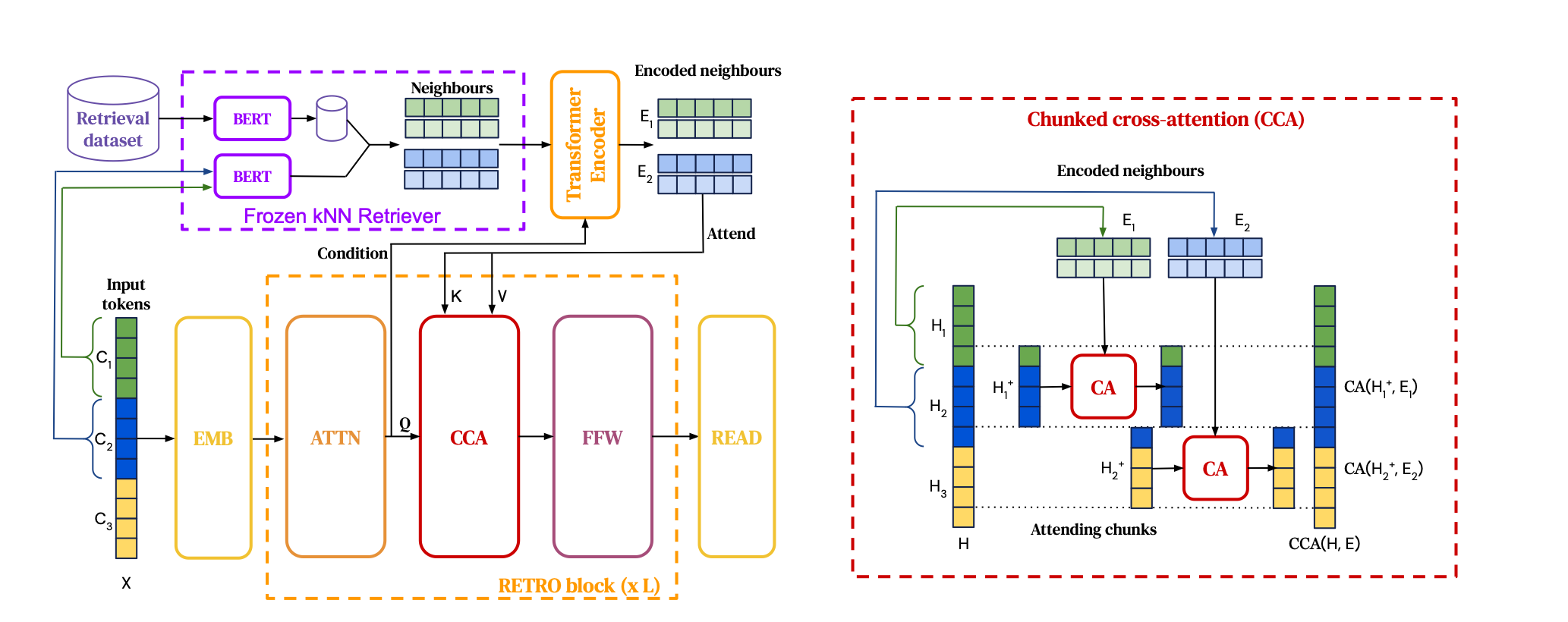
Retrieval-Enhanced Transformer (RETRO) is an autoregressive language model enhanced by retrieval capabilities, trained with a next-token prediction objective.
RETRO combines a frozen BERT retriever, a differentiable encoder, and a chunked cross-attention mechanism. Retro achieves performance comparable to GPT-3 on the Pile test sets, using 25× fewer parameters.
RETRO operates by dividing the input sequence into contiguous token chunks. For each chunk, it retrieves text similar to the preceding chunk from a database to enhance the predictions of the current chunk. Consequently, the probability of predicting the next token is contingent not only on the previously generated tokens but also on the context retrieved from the earlier chunks.
In contrast to REALM, RETRO does not train the retreiver and use pre-trained frozen BERT model. However, they invested into scaling the retrieval database to trillions of tokens, what is typically consumed during training.
To approximate k nearest neighbors or kNN, RETRO uses the SCaNN library, which is efficient, operating in O(logN) time.
Retrieved passages are integrated using an encoder-decoder transformer architecture via a cross-attention mechanism. Specifically, for each chunk 𝐶, the 𝑘 retrieval neighbors are fed into a bidirectional transformer encoder, conditioned on the activations of chunk 𝐶 through cross-attention layers. This allows the representations of the retrieval encoder to be modulated by the retrieving chunk in a differentiable fashion, yielding a fully encoded set. Next, each RETRO block uses chunked cross-attention or CCA, where the representation of the last token in the previous chunk is included in the next chunk (you can have a look at the paper if you are interested; I think they did that to allow information flow between chunks). They did a good job to illustrate it - cf figure below:
As RETRO utilizes frozen BERT embeddings, it circumvents the need to frequently recompute embeddings across the entire database during training.
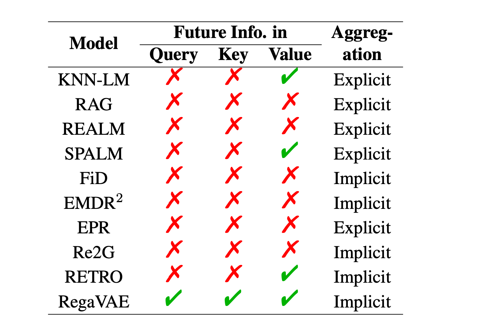
It should be stressed, as will be discussed later, that RETRO, in contrast to FiD, incorporates future information or continuation in the values. In fact, RETRO’s database takes the form of a key–value memory. Each value consists of two contiguous chunks of tokens, denoted as \([N, F]\), where N is the neighbor chunk used to compute the key, and F is its continuation in the original passage. The BERT embedding of N is averaged to form the associated key, denoted as \(\text{BERT}(N)\). The storage structure is represented as \(R(N) \rightarrow [N, F]\), where \(N\) is a chunk from one of the indexed documents, \(F\) is the immediately following chunk, and the key \(R(N) \in \mathbb{R}^d\) is the embedding of \(N\).
While RETRO adds future tokens in the value part , RegaVAE extends the inclusion of future information to the query and key. This comprehensive integration of future information plays a crucial role in determining the similarity. Jingcheng Deng et al. advocate that effective retrieval should consider not just the current semantic information but also future semantic insights. Including future information while retrieving passages promises enhanced fluency.
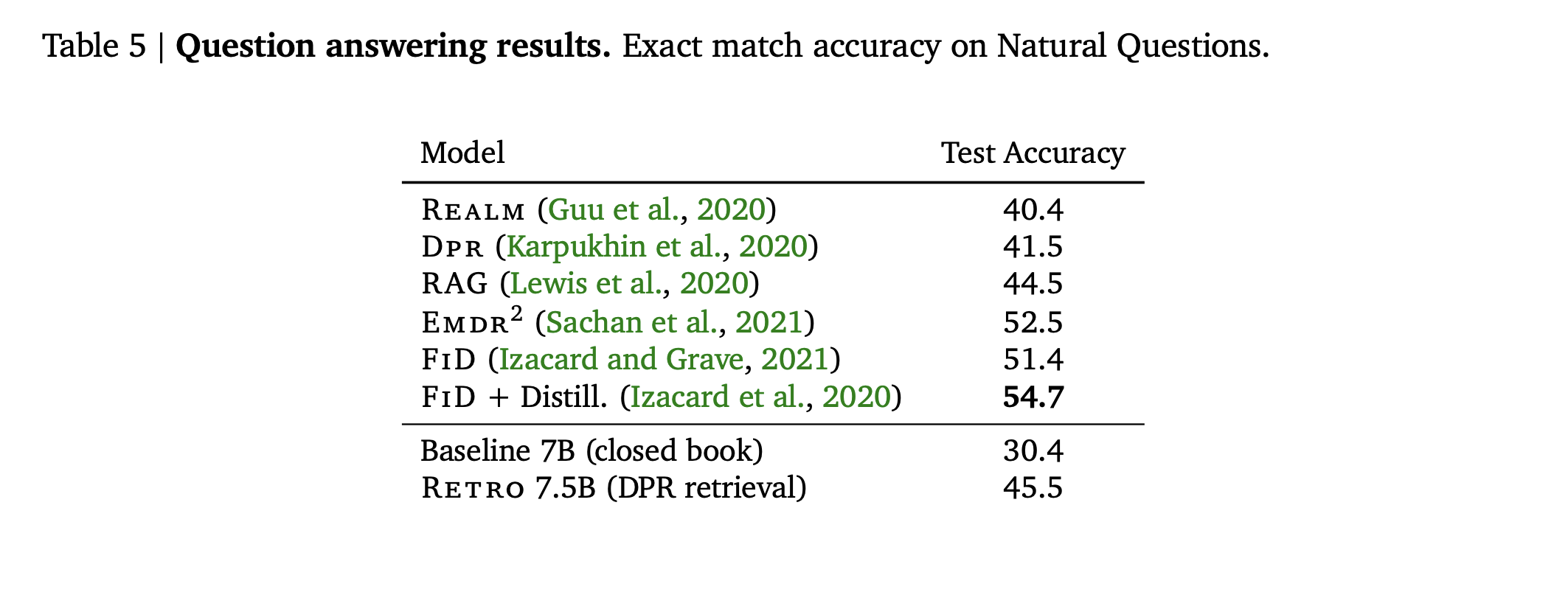
Finally, RETRO was fine-tuned on the Natural Questions dataset and demonstrated competitive results when compared with earlier models like REALM, RAG, and DPR. However, it didn't perform as well as the more recently developed model FiD.
As discussed earlier, having access to an external, non-parametric knowledge source through a retrieval-augmented architecture effectively separate memorization from generalization.
ATLAS is a pre-trained retrieval-augmented language model that differs from REALM. The retrieval module in ATLAS is based on the Contriever (retriever trained with contrastive learning and without supervision). The Contriever utilizes a dual-encoder architecture, where the query and documents are independently embedded using a transformer encoder. In order to produce a sentence representation for each query or document, ATLAS uses average pooling over the outputs of the last layer. The similarity between a query and a document is determined by calculating the dot product of their respective embeddings.
In ATLAS, the language model employs the Fusion-in-Decoder (FiD) approach. The paper discusses four distinct loss functions used in the model's training, discussed below.
ATLAS capitalises on feedback signals from the language model to help the retriever perform better its job, without the need to annotate documents.
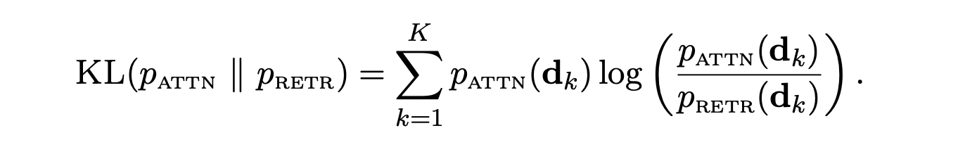
Building on the observations of Izacard et al. (2021), cross-attention scores between input documents and the generated output can be used as a proxy for the importance of each document in the generation process. The relevance of a text segment is determined by its contribution to answering the question. In simpler terms, the proposal is to train the retriever by teaching it to approximate the reader's attention scores, with the relevance of a text segment being directly linked to the level of attention its tokens receive.
In this framework, the teacher is the reader module, and the student is the retrieval module. Only the parameters of the retriever are updated by applying a StopGradient operator (which is widely available in most modern DL frameworks). You can have a look at either the original paper who proposed the idea Izacard et al. (2021) or ATLAS (2023) for more details about the scoring and training details.
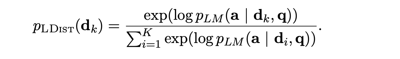
The EMDR2 loss is employed to train the retriever. It involves the calculation of the negative log-likelihood of the language model's predictions, considering both the query and the retrieved documents.

This loss function aims to train the retriever to predict the potential improvement each document can bring to the language model's prediction accuracy, given a query. It minimizes the KL-divergence between the retriever's document distribution and the language model's posterior document distribution, which is conditioned on a single document and a uniform prior. Below, a is the corresponding output of the query q.
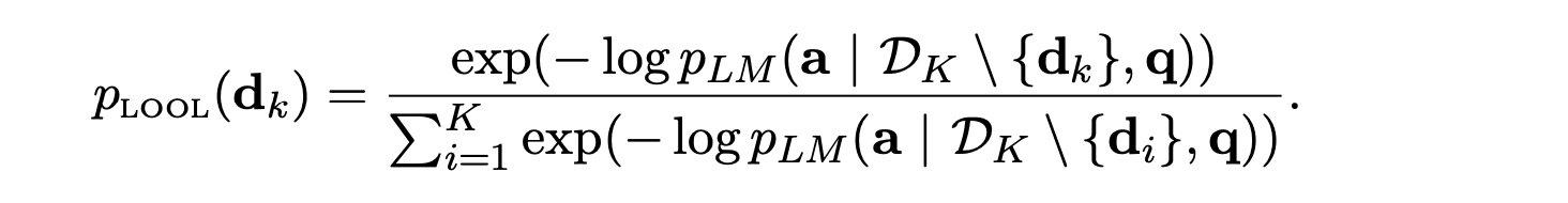
The final loss function trains the retriever to assess how the exclusion of each top-k retrieved document affects the language model's prediction. It calculates the log probability of the output for each subset of k-1 documents, using the negative value as the relevance score for each document, and then minimizes the KL-divergence between the distribution below and the retriever's distribution, this will help the retriever know, through distillation, how much a document does not contribute for the prediction. You can have a look at the paper for more details.
With only 11B parameters, ATLAS achieves 42.4% accuracy on the Natural Questions dataset using only 64 training examples, surpassing the 540B parameter model PaLM. In a full dataset setting with a Wikipedia index, ATLAS sets a new SOTA benchmark with 64.0% accuracy, an 8.1 point improvement over existing models.
As discussed in an earlier section, Variational Autoencoders (VAEs) aid in regularizing latent representations for natural language, leading to an isotropic latent space. In such a space, representations of randomly sampled tokens exhibit low cosine similarity and do not cluster in a specific direction (degeneration problem).
OPTIMUS is a large-scale language VAE model, the first of its kind to combine the strengths of VAE, BERT, and GPT, supporting both natural language understanding and generation tasks.
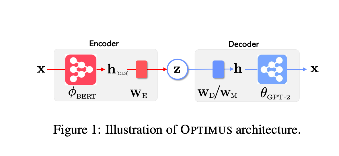
Regarding its model architecture, OPTIMUS employs Transformer-based encoders and decoders. Specifically, it utilizes a pretrained BERT for the encoder and a retrained GPT-2 for the decoder. To capture the bottleneck of a sentence (since their reconstruction is at the sentence level, not the token level), OPTIMUS uses the last [CLS] token's contextual representation as the sentence's hidden representation.
A trainable projection matrix is then used to obtain the bottleneck z for the VAE. z is subsequently fed to the decoder to reconstruct the input x. Note that we don't usually train Transformers-based encoder-decoder models in an autoregressive way (otherwise we have the same issue as RNN), or in other words, we don't produce token by token after each forward step during training, we usually use teacher forcing/masking to train in parallel (basically by shifting outputs by one token to the right; effectively learning generate one token at a time) as we already know the output embeddings. If you want to learn more about how GPTs emerged and how they are being trained, have a look at my ebook.
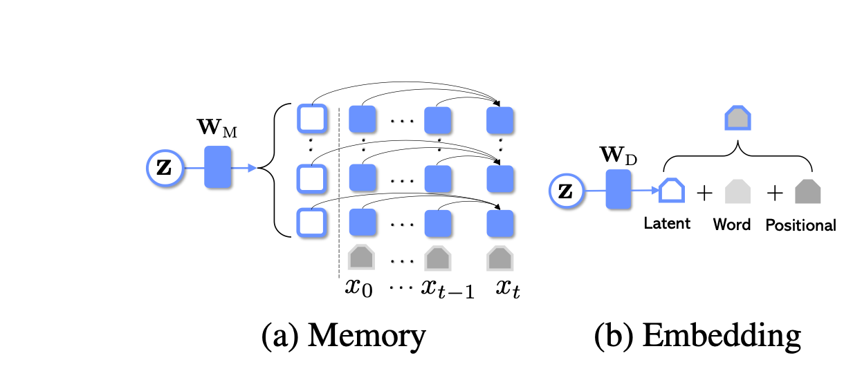
The paper proposes two methods for integrating the bottleneck z into GPT-2:
The paper observed that using Memory is significantly more effective than Embedding, and combining both approaches yields slightly better results. This is logical, as the Memory approach allows attending to the bottleneck at every layer.
Compared to models like BERT, OPTIMUS offers a more structured, smooth, and semantically rich latent space due to the incorporation of the prior distribution in training. When compared with generative decoders, OPTIMUS achieves lower perplexity than GPT-2 on standard benchmarks.
Transformer-based Conditional Variational Autoencoder for Controllable Story Generation presents a novel approach to neural story generation. The authors focus on enhancing the controllability of text generation in long text settings, using large-scale latent variable models, particularly the Variational Autoencoder (VAE) and Conditional Variational Autoencoder (CVAE).
This paper differs from OPTIMUS, specifically in that they consider both VAE and CVAE. Additionally, this paper utilizes GPT2 for both the encoder and decoder, whereas OPTIMUS employed BERT for the encoder and GPT2 for the decoder.
To obtain a latent code, as represented below, they define an attention-average block to merge a variable length sequence of vectors into a single vector. This average block essentially performs multi-head self-attention, using a learnable single query \( Q = q_{\text{avg}} \in \mathbb{R}^d \), and \( K = V \) taken as the variable length sequence of vectors from the last blocked self-attention layer. The output vector representation is then passed to linear layers to predict prior and posterior distributions, respectively, see figure below.
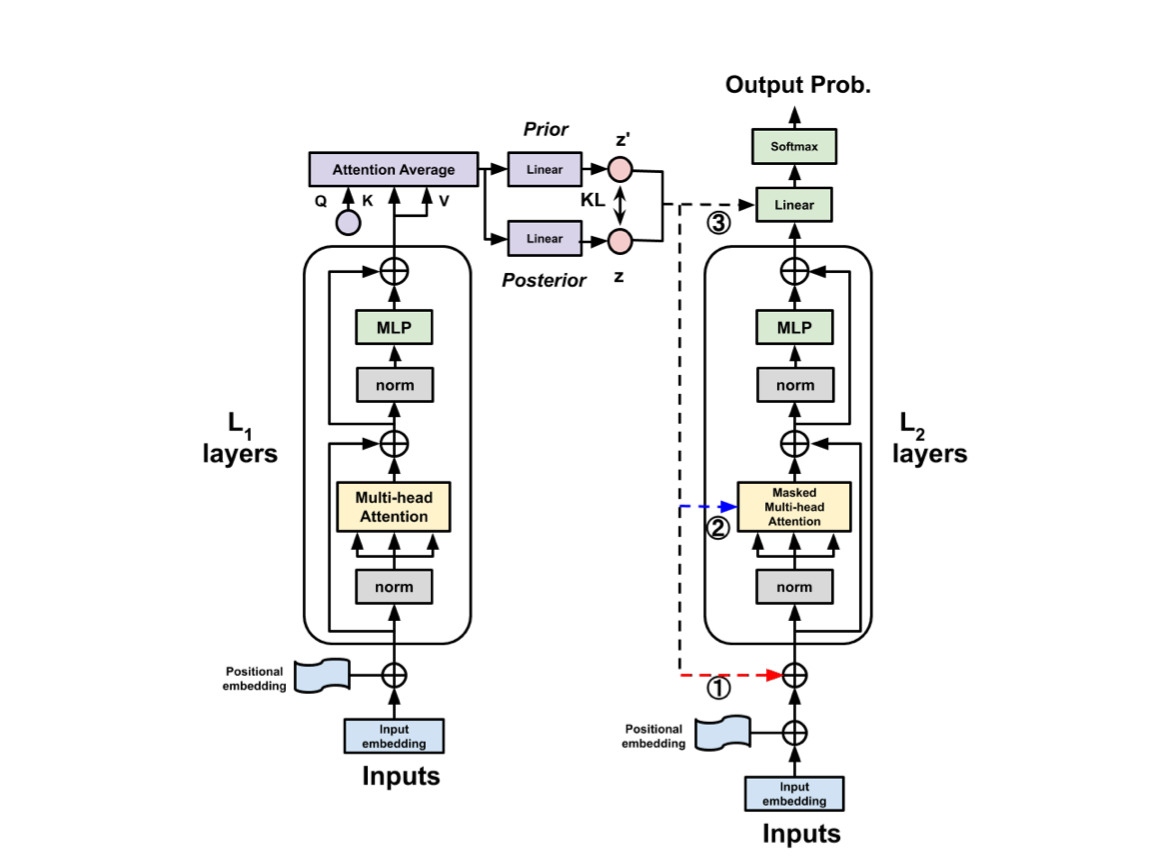
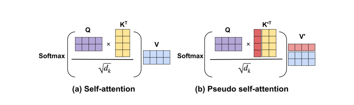
In order to inject the latent code into the decoder, they investigated three methods: First, pseudo self-attention (PSA), which injects the latent code \( z \) on a per-layer basis. Specifically, \( z \in \mathbb{R}^d \) is projected into \( z_L \in \mathbb{R}^{d \times L} \) through a projection matrix, allowing it to be split into \( L \) vectors \( [z_1, \ldots, z_L] \), with \( z_l \) being fed into the \( l \)-th blocked self-attention layer. In other words, the keys and values are augmented beyond vanilla self-attention. This is illustrated below.
Additionally, the latent representation of the input sequence can also be used with the pre-softmax logit vector. Essentially, the vanilla hidden representation is added to a latent vector, obtained from projecting the latent code summarizing the sequence into a space having the same dimension as the vocabulary size. Finally, the latent code can also be added to the word and position embeddings.
Transformer-based latent variable models take a very interesting approach, which consists of marrying CVAE and GPT2 to enhance controllable text generation while maintaining state-of-the-art generation effectiveness. We will discuss later how this leads to more interesting approaches in retrieval-augmented models.
The ADAVAE paper posits that language models based on VAEs require excessive resources. For instance, OPTIMUS necessitates the fine-tuning of two pretrained models (GPT2 and BERT), which is resource-intensive. They proposed a VAE framework, ADAVAE, empowered with adaptive GPT-2s, marking the first "big VAE'' model with unified parameter-efficient PLMs that can be optimized with a minimum of trainable parameters. Parameter-efficient fine-tuning involves freezing certain parameters while only training a subset or alternatively, introducing additional parameters. You can have a look at one of my previous articles to learn more about that.
Essentially, the paper capitalizes on the fact that VAEs offer powerful generative modeling capabilities and a rich latent representation space. ADAVAE consists of two adaptive, parameter-efficient GPT-2s in the encoder, where the causal mask is removed to fully perceive the context, including future and previous tokens.
Specifically, they added additional adapter components between the feedforward layers and the output of an attention block in these GPT-2s.
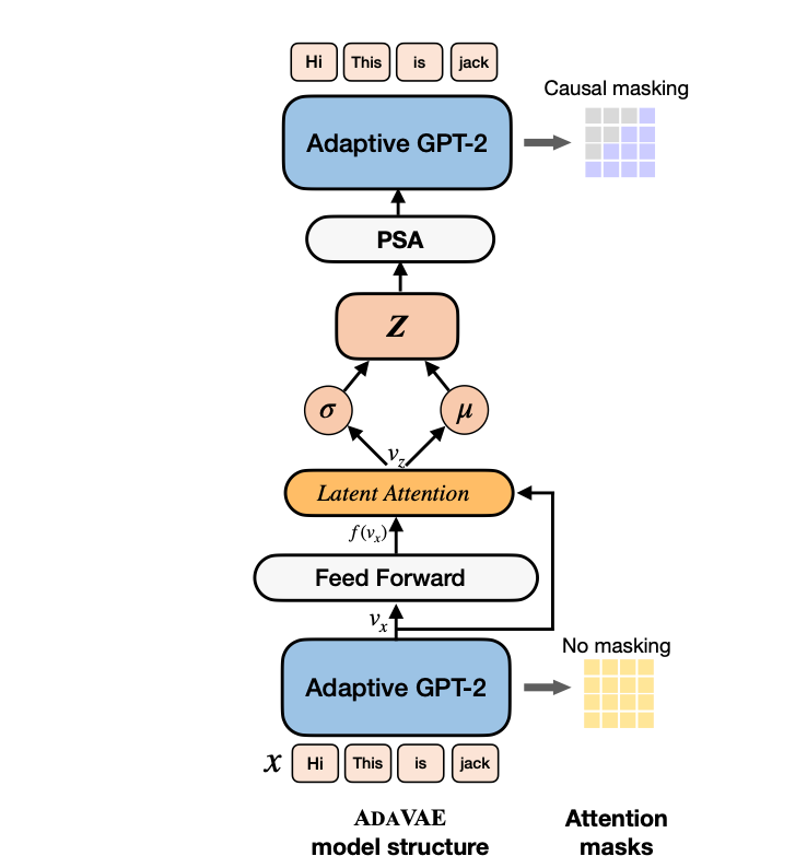
The paper introduces Latent Attention to generate a meaningful latent space. Specifically, to obtain the latent vector \( \mathbf{v}_z \), the last hidden state \( \mathbf{v}_x \) from the encoder is adopted, and
$$\begin{align*}
Q_z &= \mathbf{E}, \\
K_z &= f(\mathbf{v}_x), \\
V_z &= \mathbf{v}_x, \\
\mathbf{v}_z &= \text{Attention}(Q_z, K_z, V_z),
\end{align*}$$
where \( \mathbf{E} \) is an identity matrix of the same size as \( \mathbf{v}_x \), \( f(\cdot) \) is a linear transformation \( \mathbf{v}_x \) to the key vector space, and \( \mathbf{v}_z \) is derived from the attention operation between \( Q_z \), \( K_z \), and \( V_z \). The latent vector \( \mathbf{v}_z \) is then used to reparameterize the mean \( \mu \) and variance \( \sigma \) of \( Z \):
$$\begin{align*}
\mu &= f_\mu(\mathbf{v}_z), \\
\log(\sigma) &= f_\sigma(\mathbf{v}_z), \\
z &= \mu + \sigma \odot \varepsilon, \quad \varepsilon \sim \mathcal{N}(0, \mathbf{I})
\end{align*}$$
To utilize the sentence bottleneck for feeding the generator, two methods were investigated: Add to Memory (AtM), which projects \( z \) to both attention key and value spaces via a unified linear layer \( f(\cdot) \), and concatenates them with the key and value vectors in each attention layer. The other method is Pseudo Self-Attention (PSA), similar to AtM, discussed earlier, which ensures that \( \mathbf{t}_k \neq \mathbf{v}_z \). You can have a look at the paper for more details.
ADAVAE achieves SOTA performance in language modeling and comparable performance in classification and controllable generation tasks, with only 14.66% of parameters activated.
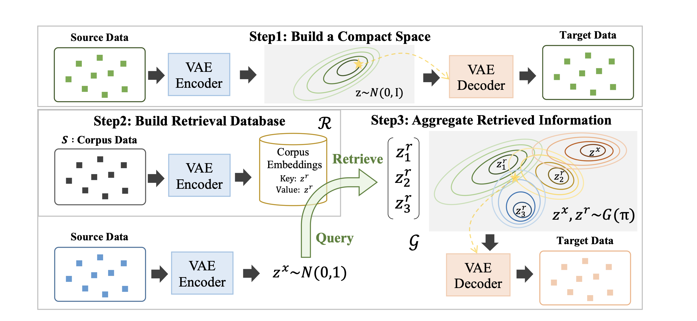
RegaVAE leverages a compact latent space using variational regularization and is designed to map inputs into a Gaussian latent space capturing current and future information using conditional VAE. This mapping is crucial as it uses the metric properties of this space to perform similarity searches, enabling retrieval of information within the latent space.
Compared to other models, RegaVAE's latent representations, which are utilized for retrieval, encompass both current and future information. This is achieved by training a compact space using a Conditional Variational Autoencoder (CVAE), ensuring that the latent space inherently contains information about future tokens without the explicit addition and encoding of these tokens. More specifically, RegaVAE used DELLA, for obtaining such space.
The aggregation approach in RegaVAE also differs from other models. It employs an implicit aggregation model using a mixture of Gaussians. Specifically, each encoded passage representation follows a Gaussian distribution. Consequently, they consider using a Gaussian mixture distribution to effectively and implicitly combine/aggregate the query representation with the retrieved passage. This is illustrated below.
Similar to other frameworks, RegaVAE periodically updates the retrieval database index at fixed intervals during the training process.
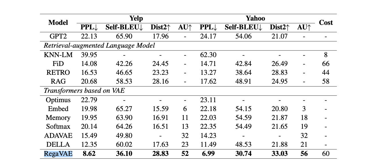
RegaVAE surpasses traditional retrieval-based generative models in several aspects. It excels not only in the quality of generated content but also in reducing hallucinations, a common issue in generative models where the model generates nonsense.
Plain Transformers do not inherently possess knowledge about the positions (or timing) of tokens, and very often, the order of words affects the meaning. To compensate for the absence of a cyclic structure inherent in RNNs, which naturally capture positional information, Transformers employ positional encoding.
Position itself carries information, and it's crucial to include this in the model; otherwise, our model becomes permutation invariant. This means that \( f_{\theta}(\pi(x)) = f_{\theta}(x) \), where the function \( f_{\theta} \) represents the model's output, and \( \pi(x) \) represents a permutation of the input \( x \).
Absolute Positional Encoding involves augmenting the input embeddings with absolute positional encodings \( p = (p_1, \ldots, p_n) \) through addition, rather than concatenation, to avoid issues with dimensionality and computational burden. The process is defined as \( x_i = x_i + p_i \), where \( p_i, x_i \in \mathbb{R}^d \).
There are several choices for positional embeddings. One approach is to use fixed sinusoidal encodings, generated using the sine-cosine rule. The formula is as follows:
$$
P(i, 2j) = \sin\left( \frac{i}{10000^{2j/d}} \right), \quad \text{and} \quad P(i, 2j+1) = \cos\left( \frac{i}{10000^{2j/d}} \right)$$
where \( d \) is the dimension of the embedding space. The obtained matrix assigns to each token a vector representation holding information about its position.
Another approach is to use learnable encodings through backpropagation.
One drawback of using absolute positional encoding is that it does not easily generalize to contexts larger than the model was trained on, as the positional encoding strongly depends on the sequence's length to model positional information. This limitation has led to the proposal of alternative methods like Relative Positional Encoding (RPE) and Rotational Positional Encoding (RoPE), which are widely used today and also consider relations between neighboring word positions.
The relative distance between tokens at positions often matters more than their absolute positions. This was highlighted by Shaw et al. (2018), who built on the idea that time lags, represented as \((j-i)\), are more critical for accurate predictions than absolute positional information. This observation gave rise to the concept of Relative Position Encoding (RPE), which introduces a novel approach to integrating positional information into models.
Unlike APE, which modifies the input embedding directly, RPE "injects" positional information where it is most needed: within the attention module.
RPE involves encoding the relative position between tokens \(i\) and \(j\) into vectors. This is integrated into the self-attention module of the Transformer. The modified self-attention mechanism now contains extra parameters \(p_{ij}\) for every pair of query \(i\) and key \(j\), representing their pairwise relative position information. Formally, this can be described as:
$$\begin{align*} f_q(x_m) &= (W_q x_m) \\
f_k(x_n, n) &= W_k \left( x_n + p^K_{r} \right) \\
f_v(x_n, n) &= W_v \left( x_n + p^V_{r} \right) \end{align*}$$
\(P^V = (p^V_{-k}, \ldots, p^V_{k}) \quad \text{and} \quad P^K = (p^K_{-k}, \ldots, p^K_{k}) \quad \) are trainable matrices and \( p^V_{i}, p^K_{i} \in \mathbb{R}^{d}\). To manage the complexity and enhance the model's ability to generalize, the number of parameters are clipped, that is, above \(r = clip(m − n, k)\), where \(clip(x, k) = max(−k, min(k, x))\). The clipping ensures that the model only considers relative position information for tokens that are at most k tokens away from each other and reduce trainable parameters and allows the model to generalize to unseen sequence lengths more effectively.
Additionally, relative position encoding can be either shared across attention heads or implemented separately for each head, offering a degree of flexibility in modeling different types of positional relationships.
Finally, it is interesting to see that the method of encoding relative positions now resembles the mechanism of attention as if we were concatenating the input embeddings with the positional embeddings, something we avoid practically [for a rough proof ,cf question (c) in https://inst.eecs.berkeley.edu/~cs182/sp23/assets/section/dis10/sol10.pdf, which take into account the general orthogonality of large vectors in high-dimensional spaces + https://arxiv.org/pdf/2104.09864.pdf].
RPE enables the model to learn how to incorporate relative distances through backpropagation. Essentially, the model learns to add a bias or clue to the self-attention module. Several Relative Position Encoding methods have been proposed beyond the one presented by Shaw et al. (2018), for example, Transformer-XL reparametrized vanilla attention score to introduce a new form of relative positional encodings using sinusoid encoding matrix and adding trainable parameters for relying on relative positional information. The updated attention score is shown below, you can have a look at the paper for more details.
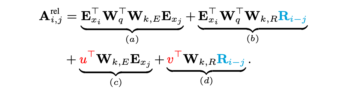
Position encoding plays a crucial role in transformer architectures, as it provides vital information about the order and relative positions of elements in a sequence. Initially, transformers utilized absolute positional encoding, which directly represents the specific position of each token in a sequence. This approach included methods like sinusoidal encoding. Over time, the concept evolved into relative positional encoding, which focuses more on the relative distances and relationships between tokens, offering a more dynamic understanding of sequence context. Relative positional encodings are particularly adept at capturing the relevance and relationships between words, often outperforming absolute positional encodings in this regard.
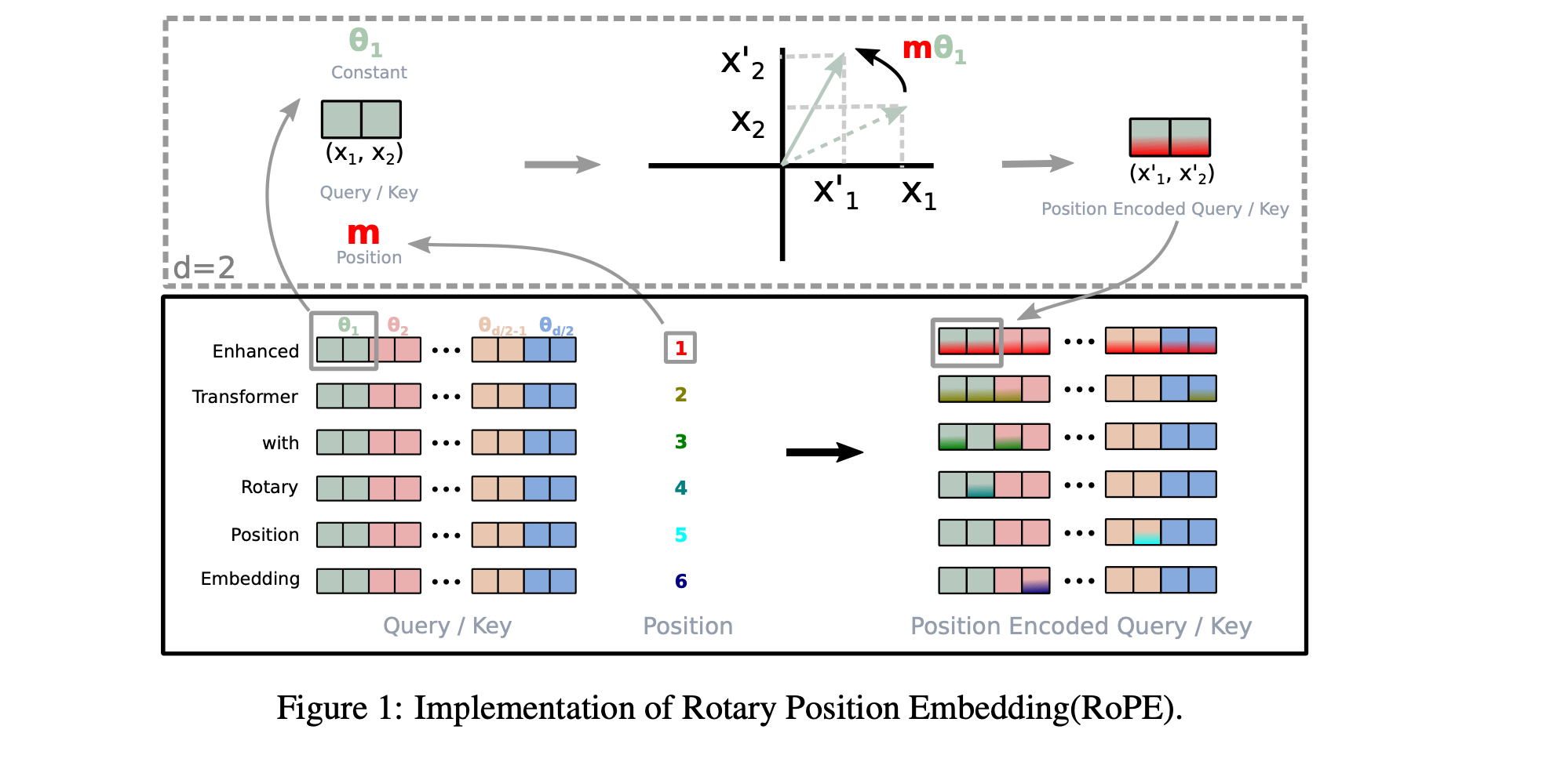
RoPE uniquely combines the benefits of absolute and relative positional information. It encodes absolute positions using a rotation matrix while simultaneously integrating relative position dependencies into the self-attention mechanism of transformers. This method is notable for its flexibility in handling variable sequence lengths and its ability to model the decaying influence of tokens with increasing relative distance. Its effectiveness has been demonstrated in various LLMs, including Llama and PaLM.
Formally, RoPE identify the embedding space and hidden representations vector space as complex vector spaces, specifically, the query and key vectors in RoPE are represented as follows:
\begin{align*}
f_q(x_m, m) &= (W_q x_m) e^{i m \theta} \\
f_k(x_n, n) &= (W_k x_n) e^{i n \theta}
\end{align*}
The dot product between the query vector and the key vector depends only on the relative distance m−n, with the function \(g(x_m,x_n,m−n)\) representing this relative position dependency. The equations for this relationship are:
$$\begin{align*}
\langle f_q(x_m, m), f_k(x_n, n) \rangle_R &= \text{Re}(\langle f_q(x_m, m), f_k(x_n, n) \rangle_C) \\
&= \text{Re}(W_qx_m (W_k x_n)^* e^{i \theta (m - n)}) \\
&= g(x_m, x_n, m - n)
\end{align*}$$
where \(Re[·]\) is the real part of a complex number and \(W_{k \times n}^*\) represents the conjugate complex number of \(W_{k \times n}\).
For a general form where the dimension d is even, the rotary position embedding is extended:
$$\begin{align*}
f_{\{q, k\}}(x_m, m) &= R_d^{\Theta, m} W_{\{q, k\}} x_m
\end{align*}$$
The rotary matrix \(R_d^{\Theta, m}\) is defined as a block diagonal matrix with 2D rotation matrices along the diagonal:
$$\begin{align*}
R_d^{\Theta, m} = \begin{pmatrix}
\cos m \theta_1 & -\sin m \theta_1 & 0 & \cdots & 0 \\
\sin m \theta_1 & \cos m \theta_1 & 0 & \cdots & 0 \\
\vdots & \vdots & \ddots & \vdots & \vdots \\
0 & 0 & \cdots & \cos m \theta_{d/2} & -\sin m \theta_{d/2} \\
0 & 0 & \cdots & \sin m \theta_{d/2} & \cos m \theta_{d/2}
\end{pmatrix}
\end{align*}$$
Overs the years/months, several methods capitalised on the benefits of rotary positional embedding, more recently, YaRN (Yet another RoPE extensioN method) [2023]. YaRN extends the context limit of LLaMA-2 models to 64k/128k tokens, a substantial increase from the original 4k token limit.
Scaling laws (Kaplan et al. and Chinchilla) have demonstrated that increasing model parameters, among other factors, can lead to more capable models. In other words, performance and model parameter size follow a power-law relationship. However, scaling comes with key challenges:
To address these challenges, a plethora of work have been conducted to make LLMs more efficient:
If you found a mistake, please let me know.